What is a Descriptive Statistics Report?
Descriptive statistics, as the name implies, refers to the statistics that describe your dataset. For a large dataset, it gives you a bite-sized summary that can help you understand your data. Imagine this as being the Resumé of the data you are going to work with, it tells you what your data holds. Statisticians often need to create a descriptive statistics report as a first step before diving into rigorous analytics and inferential statistics of a data.
In this tutorial I will be going over how to create a descriptive statistics report in R for a complete dataset or samples from within a dataset. We’re going to show you a couple of different approaches to how to find descriptive statistics in r, using functions from both base R and specialized packages.
How to Interpret Summary Statistics in R
A descriptive statistics report normally comprises of two components, measures of central tendency and the variability of data.
Central tendency, as suggested by the name, refers to the tendency or the behavior of values around the mean of the dataset. Variability, on the other hand, refers to the scatter or the spread of values in the set. These two components give you a fair estimate of what your data means. There are a number of parameters included in these components that a descriptive statistics report comprises of.
Before I begin explaining how you can obtain a descriptive statistics report in R, I’ll first explain what each of these measures mean. It’s crucial that your understanding of each of these parameters is solid because it serves as a foundation to advanced data analytics.
- Mean– It is obtained by averaging all the numerical observations in a dataset.
- Median – It is the midpoint that separates the data evenly into two halves. The median, unlike the mean, is not sensitive to extreme values and outliers.
- Mode – It tells which observation occurs most frequently in the dataset. Notice that the last two measures only apply to numerical data whereas mode can be taken for nominal data as well.
- Range– It’s the difference between the extremes of your data.
- Standard Deviation– It estimates the variation in numerical observations.
- Variance– It measures how spread out or scattered values are from the mean. Standard deviation squared is essentially the variance.
- Skewness– It speaks about how symmetric your data is around the average. Depending on where the extreme values lie, your data may have a positive or negative skew.
- Kurtosis– It is a visual estimate of the variance of a data. Your normal distribution curve may be peaked or flat, kurtosis estimates this property of your data.
- Interquartile Range– It divides the data into percentiles. Interquartile range is often a more interesting statistic, it is the central 50% of the data.
You can see that some parameters in descriptive statistics are more significant when data isn’t perfectly normal, such as skewness and variance. In fact, statisticians often work with data that isn’t completely neat and easy to handle. Your data may have outliers, or it may even peak twice (a bimodal distribution). However, statistics gives you tools for studying such data and adjusting it for use. One of the decisions statisticians sometimes need to make is whether to keep outliers or remove them. Studying your data closely gives you answers to all such questions.
Now that you have an understanding of what a descriptive statistics report shows, I can begin to explain how you can obtain one in R.
Generating Descriptive Statistics in R
In this tutorial,
I’ll be using an in-built dataset of R called “warpbreaks”. We’ll first start
with loading the dataset into R.
# import data for descriptive statistics in R tutorial
> data(warpbreaks)
The summary function in R is one of the most widely used functions for descriptive
statistical analysis. It gives you information such as range, mean, median and interpercentile ranges.
# summary code in r (summary statistics function in R)
> summary(warpbreaks)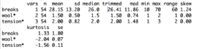
R also allows you to obtain this information individually if you want to keep the coding concise. For instance, the “mean()” function can be used to get the average of your data. However, you need to enter a list in such functions instead of a data frame as could be used with “summary()”.
# Example of summary statistics in R (for specific field)
> mean(warpbreaks$breaks)
This tells you the average breaks that happen during weaving. You can calculate median(), range(), length(), min() and max() in a similar manner. However, in order to obtain measures of variability you need to install additional packages. The skew, for instance, can’t be calculated directly using an in-built function of R. The “moments” package gives you some very convenient methods of doing this. Your code to individually calculate skewness and kurtosis should look like this.
# Summary statistics in R (r descriptive statistics tutorial)
> install.packages(moments)
> library(moments)
> skewness(warpbreaks$breaks)
> kurtosis(warpbreaks$breaks)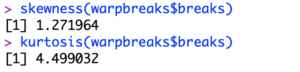
Other Tools for Descriptive Statistics in R
Another package of R called “psych” can be used to obtain a more detailed report through the “describe()” function. The describe function gives you some measures of variability as well which the “summary()” function does not.
# Descriptive statistics in R Tutorial (Altenative Options)
> library(psych)
> describe(warpbreaks) Sometimes, data is divided into groups and you may want categorical statistics for it. Fortunately, R allows you to do that in a number of ways as well. I personally find the “aggregate()” function to be the easiest method of going about it. The dataset I’m using, “warpbreaks”, has data for two different kinds of wools, A and B, using the “aggregate()” function you can calculate statistics for each wool separately.
# Aggregate Function Example: R Summary Statistics by Group
> aggregate(breaks~tension , data= warpbreaks, mean)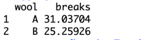
Aggregate – Get R Summary Statistics by Factor
Finally, visualizing data is an important part of understanding the patterns within statistical data. Statisticians, especially financial statisticians, are often interested in knowing whether their data fits a normal distribution. You can check that using the “qqnorm()” function.
# using qqnorm to check for normality
> qqnorm(warpbreaks$breaks)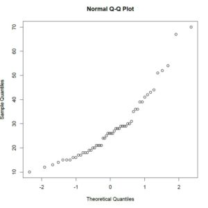
Finally, frequency tables can be used to determine if your data follows a pattern or a relationship against another variable, you can learn about contingency tables in R here .
Going Deeper…
Interested in Learning More About Categorical Data Analysis in R? Check Out
Graphics
Tutorials
- How To Create a Contingency Table in R
- How To Generate Descriptive Statistics in R
- How To Create a Histogram in R
- How To Run A Chi Square Test in R (earlier article)
The Author:
Syed Abdul Hadi is an aspiring undergrad with a keen interest in data analytics using mathematical models and data processing software. His expertise lies in predictive analysis and interactive visualization techniques. Reading, travelling and horse back riding are among his downtime activities. Visit him on LinkedIn for updates on his work.