Real world stock price analysis involves a lot of repetitive work, such as screening many candidates to pick the right stocks or running a weekly update on your portfolio. Fortunately, you can use R scripts to automate a lot of the basic data extraction, manipulation, and plotting… giving you more time to research and think about where to invest. In the time it takes for you to get a cup of coffee, R can easily churn out an entire analysis of your portfolio or a list of stock symbols.
This is also a good introduction to using R for practical analysis. Here are few things that stock market analysis in R can teach you:
- Using R’s Built In libraries and packages to quickly pull back data
- How to generate time series charts – automatically (without tedious formatting in Excel)
- If you’re interested, how to do deeper statistical analysis of time series data
One of the challenges of stock market analysis is the volume of stock price data is gigantic and often behind a paid service. The good news is R has libraries for connecting to many free services which can help support your analysis (particularly for academic and non-commercial usage). This is a huge boon to the student, junior analyst, or amateur investor….
In this tutorial we will use r programming language along with timeseries forecasting built in r packages to learn how to run a basic stock market analysis module in R-studio. We will walk through data extraction, plotting, and analysis step by step to show how the price of Apple stock changes over time using some common R packages. The same techniques can easily be applied to other stocks (just change the ticker symbol) or market indexes (if you know the ticker symbol).
Import Historical Data Directly from Yahoo Server:
Let us import some important libraries first, and right after we will use the “pdfetch” package to directly pull historical data from AAPL as a data frame object in the R-studio Global Environment.
# Load Library
library(quantmod)
library(tseries)
library(timeSeries)
library(forecast)
library(pdfetch)
And we can go ahead and grab the stock data for everyone’s favorite mobile phone manufacturer…
AAPL <- pdfetch_YAHOO ('AAPL')After running the above libraries and R code, we will get Apple’s historical prices as a data frame in the R-studio Global Environment. Since it is good form to run a descriptive statistics procedure on any new data set… and peek at the first set of records, let’s go ahead and do that now. We will use the summary() function and the head() function to accomplish this. The summary statistics will be displayed in the output console. These could also be dumped into another data frame if we were running this analysis on multiple stocks and wanted to compare stocks to see which ones had generated the highest returns or had the most volatility.
R CODE:
summary <- as.data.frame(summary(AAPL))
head(summary)
tail(summary)
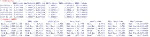
Here in the tutorial, we can use the head and tail functions to check different portions of the data set in the output console. The data set summary has also been added as a data frame in the Global Environment, which we can export as a spreadsheet if we wish.
Show Me the Money! (Stock Price Charts):
Now that we’ve got some stock price data, let’s plot it! Here’s a quick visualization tutorial that covers basic time series plotting techniques that can work for any stock price data set. First, we need to load the libraries we discussed at the beginning of this tutorial. Then after, we should narrow down the period, let us say we want to visualize the last 10-month data, and therefore you need to specify the date range by using the following codes:
Code:
chartSeries(AAPL, subset = 'last 10 month', type = 'auto',theme=chartTheme('white'))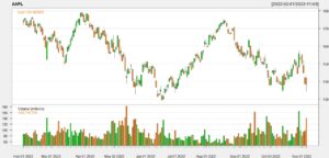
The above figures plotted all the variables of the AAPL stock over the last 10 months. If you look carefully, you can find some patterns in the stock price change, and in the next step, we will check specific features, for example, we will plot only the closing price or only the high price to see how it looks. Also, we will all have some features in the plotting so that you can get used to time series data visualization using R programming language.
So, let us plot another chart with only the adjusted closing price of AAPL from January 2022 to November 2022 and practice some feature engineering techniques to play with the time series plotting. To visualize the next plot, you should run the following codes in R-studio,
Code:
candleChart(AAPL$AAPL.adjclose, TA=c(addMACD(),
              addVo()), subset = '2022', theme=chartTheme('white'))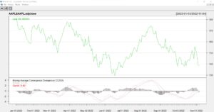
Calculate Weekly Stock Return:
We have so far discussed how to import data, how to use different libraries, and how to visualize historical stock price data using an R programming language. Now, let us use some common techniques to evaluate the characteristics of the chosen stock price.
In this section of the tutorial, you will learn how to create a new data frame and use some specific functions and libraries to calculate the weekly, monthly, and quarterly returns of a stock. We have already installed and imported the quantmod library in R-studio, and we will use this library to calculate the daily stock return first.
#  Import Last 11 month data
# Again import data from yahoo as before and create new variable.
# But here just import last 11month of data
AAPL_last_11_month  <-pdfetch_YAHOO('AAPL', from = '2022-01-01', to = '2022-11-01')
# Now select only Adjusted Closed Price from
data <- AAPL_last_11_month$AAPL.adjclose
Through the above library and functions, we can easily learn how to import data frames from live servers and create a custom data frame to use in different stock feature calculations. The date range function is very helpful for pulling any range of data and using it in the R-Studio console.
Most analysis of daily stock price returns is done with an eye to understanding volatility. We can use the hist() function to generate a histogram of these daily returns.
Stock Return Calculation:
library(quantmod)
Daily_return <- Delt(data)
hist(Daily_return)
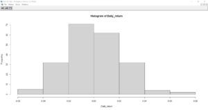
Looking at Apple’s histogram, we have a normal-ish distribution of daily returns that’s slightly skewed. The median daily return appears to be slightly negative, although there is a long tail of upside price returns which offsets these losses. This pattern is very common in stock price analysis and has been noted in other studies. A high percentage of the profits from holding a stock come from it’s performance on a handful of days.
Recap & Next Steps:
As we’ve demonstrated here, you can use R to automate pulling and analyzing data on a stock’s performance and market price. Since the example above was scripted, you could easily run it for a dozen or more stocks in a few minutes without much additional effort – just add ticker symbols. The same logic applies to situations where you need to regularly update the data, such as a weekly report or end of day update on the performance of a stock portfolio. Once you’ve built an R script, all you need to do is run the code and share the results (graphs or summary statistics).
We used a couple of key libraries to accomplish this. PDfetch provided us with a free source of financial data. This library can be used for a lot more than stock prices: it also has data from the St Louis Fed (economic indicators), Bank of England, EU sources, the World Bank, and the US Department of Labor. quantmod is a highly respected financial library which helped us generate the graphs and indicators. Other libraries (timeseries, forecast, tseries) played a supporting role within the calculations. And of course, never forget Base R’s built in capabilities with tools such as the hist() function.
Your next project in this space could be expanding this script. Perhaps to track a group of stocks – or add some custom charts. Good luck!