In this article, we are going to explore about descriptive statistics concepts related to grouped data. Descriptive statistics allow you to explore different measures of central tendencies and measure of dispersion. Here, we are going to embark on a journey to calculate the mean and median of a grouped data through R.
Mean and median are two of the measures of central tendencies which implies some important facts about the datasets that you will explore. Mean usually implies the average value of the dataset whereas median tells you about the middle value when the data is arranged (either in ascending or descending order). However, for R, there is no need to get involved in class interval or frequency distribution table formation. For this article, we are going to explore built-in dataset called “ChickWeight” that has data of how much different chick weigh based different time intervals and feed. Secondly, we will explore another dataset called “InsectSprays” that mentions effectiveness of six different insect sprays.
We will kick off by installing and loading the libraries:
Installing the Libraries
# installing the packages
install.packages("tidyverse")
install.packages("dplyr")
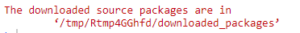
This may take a while to install. On successful installation of packages, following message will be displayed in console window:
Loading the Libraries:
# loading libraries

library("tidyverse")
library("dplyr")
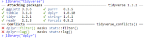
You will get the following message on successful loading of libraries in console window:
Next step is to check for a number of built-in datasets that you can explore by typing the following:
# Choosing the Dataset
data()
From the buildin datasets, I have decided to choose ChickWeight dataset by typing the following:
# Choosing the Dataset
data(ChickWeight)
Checking Data Integrity
One of the major steps in data analytics is to check for the data integrity, here are the few tricks that can help you spot any red flags prior to data analysis. It includes commands like head(), glimpse(), str().
You can do that by typing the following:
# Checking Data Integrity
head(ChickWeight)
str(ChickWeight)
glimpse(ChickWeight)
Output:
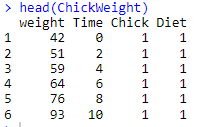
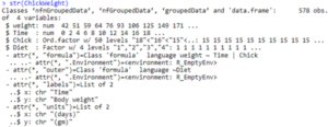
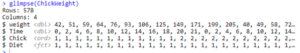
Based on the outputs, it is clearly evident that correct data-type is assigned to each column along with a firsthand overview of what the data is all about. Head() helps you get a look at first data values whereas the glimpse() will provide you with a brief outlook of different rows and columns along with data types. However for a more exploratory view, you can also choose str() that can provide with different data pertaining to classes along with different data attributes and observations.
Once we are through these pre-analysis phase, let’s head on to find the mean and median of the grouped data.
Mean and Median of Grouped Data using aggregate(), mean() and median()
With most grouped datasets, you don’t have to go through the steps of class interval creation, frequency determination, median class designation, and frequency distribution table formation if you already have a grouped dataset. However, there is an easy way out using aggregate(), mean() and median() with following syntax:
Aggregate(<dataframe>$<aggregate_variable_name>,list(<dataframe>$grouped_variable_name>,condition)
Use the following code to get mean and median of each of different diets:
# Mean Using Aggregate Function
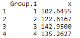
aggregate(ChickWeight$weight, list(ChickWeight$Diet), mean)
# Mean Using Aggregate Function
aggregate(ChickWeight$weight, list(ChickWeight$Diet), mean)
Use the following code to get mean and median of each of different diets:
# Mean Using Aggregate Function
aggregate(ChickWeight$weight, list(ChickWeight$Diet), mean)
Output:
# Median Using Aggregate Function
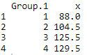
aggregate(ChickWeight$weight, list(ChickWeight$Diet), median)
Output:
Alternate Route via select() and summerise() Functions
For that, you can easily use select(), summerise(), mean(), and median() functions having the following syntax:
Select(<column_name(s)>)
summarise(<variable_name1>=condition1, <variable_name2 = condition2, …)
Here na.rm should be TRUE in order to omit any missing values that can cause bias in the analysis. So, to see the code in action, let’s say that you would like to summarize the data in terms of mean and median based on different diets while generating a tibble based on the results. For that pipe operators are the best option to have sequence of operations. Excited already, let’s use pipes by using the following code:
# Finding mean and Median using Group_by and Summarise
ChickWeight %>%
group_by (Diet) %>%
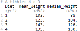
summarise(mean_weight = mean(weight,na.rm = TRUE), median_weight = median(weight,na.rm = TRUE))
Following output is displayed:
Exploring Another Dataset
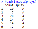
Let’s spice things up a little, let’s explore another dataset about insect’s spray and their effectiveness. The frequency is represented by the count variable whereas six different types of insect’s sprays are being considered as part of the dataset. You can access and load the dataset by typing:
#Accessing Another Dataset
data("InsectSprays")
Checking Data Integrity
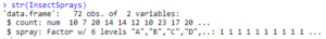
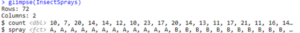
Again, for getting a glimpse of the data, repeat the same steps that you have taken in previous example.
You can do that by typing the following:
# Checking Data Integrity
head(InsectSprays)
str(InsectSprays)
glimpse(InsectSprays)
Output:
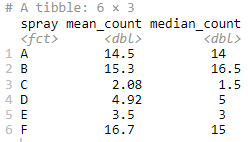
Next up, we will use the same pipe syntax to find the mean and median of the insect sprays effectiveness:
# Finding mean and Median using Group_by and Summarise
# Finding mean and Median using Group_by and Summarise
InsectSprays %>%
  group_by (spray) %>%
  summarise(mean_count = mean(count,na.rm = TRUE), median_count = median(count,na.rm = TRUE))
Output:
Based on the values obtained for spray A, the same can be visually represented through a histogram. You can use the following code to represent the mean and median effectiveness of spray A:
#Creating a subset of A
Spraysub_A <- subset(InsectSprays, spray == "A",
select=c(count))

#Installing ggplot2 package
install.packages("ggplot2")
library("ggplot2")

#Plotting Histogram
ggplot(Spraysub_A, aes(x=count)) +
  geom_histogram(color = 'darkgray', fill = 'white', binwidth = 5) +
  labs(x = 'Spray A', y = 'Effectiveness Count', title = 'Histogram of Spray A Effectiveness') +
  geom_vline(aes(xintercept = mean(Spray_A$count,na.rm = TRUE), color = 'mean'), show.legend = TRUE, size = 2) +
  geom_vline(aes(xintercept = median(Spray_A$count,na.rm = TRUE), color = 'median'), show.legend = TRUE, size = 2) +
  scale_color_manual(name = 'statistics', values = c(mean = 'red', median = 'blue'))
Output:
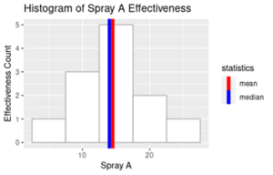
Looks a bit complex, we can discuss more about the aesthetics and visualization in our upcoming articles. However, one aspect that you might notice is that both mean and median are centrally aligned as part of the spray A effectiveness data. Besides that, frequency distribution also depicts that the Spray A effectiveness has normal distribution.
Parting Words
Values obtained for mean and median are quite identical from both methods of aggregate() and group_by(). They can be used interchangeable; however, pipe operators allow better presentation and summarization of data for the viewers. However, the same could also be calculated through the tedious steps of making class interval, calculating cumulative frequency, finding median class and finally putting them all together in a median formula. Pipe operator are a lifesaver for someone making complex data analysis calculation. On the other hand, another dataset is also analyzed in which mean and median effectiveness of sprays have been assessed using pipe operator. Alternatively, you can also visualize the mean and median of the dataset using histogram that can clearly show why they are called measure of central tendency.
Going Deeper…
If you’d like to know more about the measures of central tendencies and dispersion, you can find it out here:
Descriptive Statistics
Graphics