Statisticians often come across outliers when working with datasets and it is important to deal with them because of how significantly they can distort a statistical model.
Your dataset may have values that are distinguishably different from most other values, these are referred to as outliers. Usually, an outlier is an anomaly that occurs due to measurement errors but in other cases, it can occur because the experiment being observed experiences momentary but drastic turbulence. In either case, it is important to deal with outliers because they can adversely impact the accuracy of your results, especially in regression models.
In this tutorial, I’ll be going over some methods in R that will help you identify, visualize and remove outliers from a dataset.
Looking at Outliers in R
As I explained earlier, outliers can be dangerous for your data science activities because most statistical parameters such as mean, standard deviation and correlation are highly sensitive to outliers. Consequently, any statistical calculation based on these parameters is affected by the presence of outliers.
Whether it is good or bad to remove outliers from your dataset depends on whether they affect your model positively or negatively. Remember that outliers aren’t always the result of badly recorded observations or poorly conducted experiments. They may also occur due to natural fluctuations in the experiment and might even represent an important finding of the experiment.
Whether you’re going to drop or keep the outliers requires some amount of investigation. However, it is not recommended to drop an observation simply because it appears to be an outlier.
Statisticians have devised several ways to locate the outliers in a dataset. The most common methods include the Z-score method and the Interquartile Range (IQR) method. However, I prefer the IQR method because it does not depend on the mean and standard deviation of a dataset and I’ll be going over this method throughout the tutorial.
The interquartile range is the central 50% or the area between the 75th and the 25th percentile of a distribution. A point is an outlier if it is above the 75th or below the 25th percentile by a factor of 1.5 times the IQR.
For example, if
Q1= 25th percentile
Q3= 75th percentile
Then, IQR= Q3 – Q1
And an outlier would be a point below [Q1- (1.5)IQR] or above [Q3+(1.5)IQR].
If this didn’t entirely make sense to you, don’t fret, I’ll now walk you through the process of simplifying this using R and if necessary, removing such points from your dataset. For starters, we’ll use an in-built dataset of R called “warpbreaks”. It neatly shows two distinct outliers which I’ll be working with in this tutorial.
You can load this dataset
on R using the data function.
# remove outliers in r - import data
data("warpbreaks")
Once loaded, you can begin working on it.
Visualizing Outliers in R
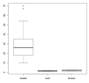
One of the easiest ways to identify outliers in R is by visualizing them in boxplots. Boxplots typically show the median of a dataset along with the first and third quartiles. They also show the limits beyond which all data values are considered as outliers. It is interesting to note that the primary purpose of a boxplot, given the information it displays, is to help you visualize the outliers in a dataset.
You can create a boxplot to identify your outliers using:
# remove outliers in R - initial boxplot
boxplot(warpbreaks)$out
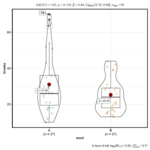
[You can also label
outliers for better visualization using the “ggbetweenstats” function
which comes with the “ggstatsplot” package. If you haven’t installed it
already, you can do that using the “install.packages” function.
Your code should look like this.
# install the package
install.packages("ggstatsplot")

# Load the package
library(ggstatsplot)

# Load the dataset
data("warpbreaks")

# Create a boxplot of the dataset, outliers are shown as two distinct points
boxplot(warpbreaks)$out

#Create a boxplot that labels the outliers
ggbetweenstats(warpbreaks,
wool, breaks, outlier.tagging = TRUE)
Finding Outliers – Statistical Methods
Now that you have some clarity on what outliers are and how they are determined using visualization tools in R, I can proceed to some statistical methods of finding outliers in a dataset.
This important because visualization isn’t always the most effective way of analyzing outliers. You can’t always look at a plot and say, “oh! this is an outlier because it’s far away from the rest of the points”. Your data set may have thousands or even more observations and it is important to have a numerical cut-off that differentiates an outlier from a non-outlier. This allows you to work with any dataset regardless of how big it may be.
Building on my previous discussion of the IQR method to find outliers, I’ll now show you how to implement it using R.
I’ll be using the quantile() function to find the 25th and the 75th percentile of the dataset, and the IQR() function which elegantly gives me the difference of the 75th and 25th percentiles.
# how to find outliers in r
Q <- quantile(warpbreaks$breaks, probs=c(.25, .75), na.rm = FALSE)
It may be noted here that the quantile() function only takes in numerical vectors as inputs whereas warpbreaks is a data frame. I, therefore, specified a relevant column by adding $breaks, this passes only the “breaks” column of “warpbreaks” as a numerical vector.
The IQR function also requires numerical vectors and therefore arguments are passed in the same way.
# how to find outliers in r - calculate Interquartile Range
iqr <- IQR(warpbreaks$breaks)
Now that you know the IQR and the quantiles, you can find the cut-off ranges beyond which all data points are outliers.
# how to find outliers in r - upper and lower range
up <-  Q[2]+1.5*iqr # Upper Range
low<- Q[1]-1.5*iqr # Lower Range
Eliminating Outliers
Using the subset() function, you can simply extract the part of your dataset between the upper and lower ranges leaving out the outliers. The code for removing outliers is:
# how to remove outliers in r (the removal)
eliminated<- subset(warpbreaks, warpbreaks$breaks > (Q[1] - 1.5*iqr) & warpbreaks$breaks < (Q[2]+1.5*iqr))
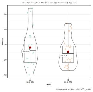
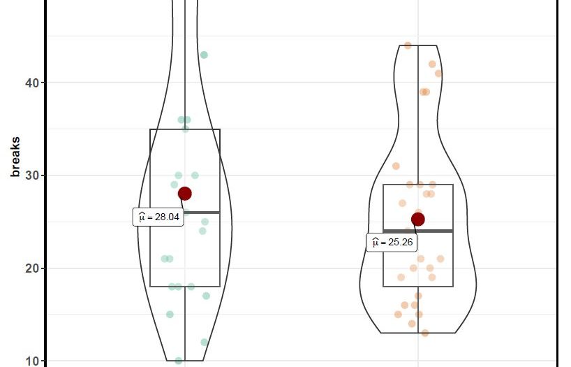
The boxplot without outliers can now be visualized:
# how to remove outliers in r - resulting boxplots
ggbetweenstats(eliminated, wool, breaks, outlier.tagging = TRUE) 
[As said earlier, outliers may or may not have to be removed, therefore, be sure that it is necessary to do so before eliminating outliers.
Other Ways of Removing Outliers
Now that you know what outliers are and how you can remove them, you may be wondering if it’s always this complicated to remove outliers. Fortunately, R gives you faster ways to get rid of them as well.
The one method that I prefer uses the boxplot() function to identify the outliers and the which() function to find and remove them from the dataset.
First, we identify the outliers:
# identify outliers in r boxplot
boxplot(warpbreaks$breaks, plot=FALSE)$out
Then save the outliers in a vector:
# how to remove outliers in r (alternative method)
outliers <- boxplot(warpbreaks$breaks, plot=FALSE)$out
This vector is to be excluded from our dataset. The which() function tells us the rows in which the outliers exist, these rows are to be removed from our data set. However, before removing them, I store “warpbreaks” in a variable, suppose x, to ensure that I don’t destroy the dataset.
# how to remove outliers in r (alternative method)
x<-warpbreaks
x<- x[-which(x$breaks %in% outliers),]
I have now removed the outliers from my dataset using two simple commands and this is one of the most elegant ways to go about it. R gives you numerous other methods to get rid of outliers as well, which, when dealing with datasets are extremely common. However, being quick to remove outliers without proper investigation isn’t good statistical practice, they are essentially part of the dataset and might just carry important information. Losing them could result in an inconsistent model.
The Author:
Syed Abdul Hadi is an aspiring undergrad with a keen interest in data analytics using mathematical models and data processing software. His expertise lies in predictive analysis and interactive visualization techniques. Reading, travelling and horse back riding are among his downtime activities. Visit him on LinkedIn for updates on his work.
