While there are many data structures in R, the one you will probably use most is the R dataframe. This is a multi-column list of information that you can manipulate, combine, and run statistical analysis on. If you are familiar with using Excel, SQL tables, or SAS datasets this will be familiar.
Lets face it. Most data starts its life as a blob. Some operational system spits out records along side the hamburgers, shipping manifests, or cases of product. These records are neatly collected somewhere in your IT organization. Logs accumulate. Dust gathers. Our job is to turn the blob into something useful.
Meet The R Data Frame
For this example, we’re going to use one of the data sets (ChickWeight) which comes with the R package. Let’s get started by pulling in the data from R’s pre-packaged libraries:
> data(ChickWeight)This is from an experiment where chickens were fed different diets and weighed over time. Each record has several attributes – what chicken, what diet, current time – and their weight. This type of data is common. Imagine someone walking around with a clipboard and entering the results into Excel. Or a quality inspector checking products on a production line.
We’re going to walk through how to examine and analyze a data frame in R. This series has a couple of parts – feel free to skip ahead to the most relevant parts. This may also be worth bookmarking for future reference…
- Inspecting your data
- Ways to Select a Subset of Data From an R Data Frame
- How To Create an R Data Frame
- How To Sort an R Data Frame
- How to Add and Remove Columns
- Cleanup – Replacing NA Values with 0
- Renaming Columns
- How To Add and Remove Rows
- How to Merge Two Data Frames
- Advanced: Create Empty Data Frame
Reviewing Contents of A Data Frame
Now that we have the data imported, we should take a look at it. That’s easy. To look at the contents of a dataframe in R, just type the name of the dataframe.
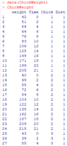
Oh my, there’s a lot of data here. There’s a better way to measure the data frame before you process it.
Getting Summary Statistics
Meet two commands:
length(ChickWeight)

nrow(ChickWeight)
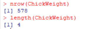
The first, length, tells us how many columns the dataframe has. Under the surface, the dataframe is a collection of what are known as “vectors”, ordered lists of values for a single variable. In this case, each vector represents a specific measurement (weight, time, chick, diet). The “length” command tells us the length of the underlying vectors in the dataframe.
The second, nrows, tells us how many rows the data frame has. We’ve got a total of 578 observations.
Another good command, which takes peek inside the contents of the dataframe, is the summary command.
summary(ChickWeight)And the results look like this:
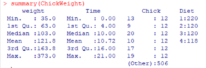
So this tells us some useful things about the contents of the data frame. First, we have quite a few chicks in this sample (the six listed plus values for 506 ones they didn’t break out). More on that in a moment. Four diets were used. And the results were spread out over time, with multiple samples per chick.
So, just how many unique chicks were in the experimental data? We’re going to combine a couple of R functions to grab that column, identify unique values using R, and count the unique values.
length(unique(ChickWeight$Chick))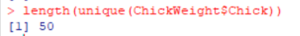
The system tells me the experiment sampled a total of 50 different birds. Lets review how this worked.
- We used the syntax DataframeName$ColumnName to grab all of the values in a particular column. Behind the scenes, this pulled off a vector of 578 data points for the next function to use.
- We fed that list of 578 data points into the unique function to boil them down to a list of unique values in that field. Behind the scenes, these are in the form of a vector as well. An ordered list of values for a single variable.
- We fed that vector into the length function to count them. And there are fifty unique values.
In the next section of this tutorial, we will examine how to select subsets of an R data frame.
If you want to skip ahead…
- Inspecting your data
- Ways to Select a Subset of Data From an R Data Frame
- How To Create an R Data Frame
- How To Sort an R Data Frame
- How to Add and Remove Columns
- Cleanup – Replacing NA Values with 0
- Renaming Columns
- How To Add and Remove Rows
- How to Merge Two Data Frames
- Advanced: Create Empty Data Frame
- Useful Functions: