The standard deviation of a sample is one of the most commonly cited descriptive statistics, explaining the degree of spread around a sample’s central tendency (the mean or median). It is commonly included in a table of summary statistics as part of exploratory analysis. If you are doing an R programming project that requires this statistic, you can easily generate it using the sd () function in Base R. This function is robust enough to be used to calculate the standard deviation of an array in R, the standard deviation of a vector in R, and the standard deviation of a data frame variable in R.
TL;DR For Finding the Standard Deviation in R
- If you’re just looking for the standard deviation in R function – that’s sd() (first topic below, with examples)
- For a better view of descriptive statistics, we recommend using the describe function from the psych library
- If you need the standard deviation for every field in an R data frame, combine the sd () and sapply() functions. Example provided below.
- Included an example of how to add error bars to a plot of data in R based on the standard deviation of a series
- Added code to download a csv file from the web or computer and run descriptive statistics on the data fields
How to Find Standard Deviation in R
You can calculate standard deviation in R using the sd() function. This standard deviation function is a part of standard R, and needs no extra packages to be calculated. By default, this will generate the sample standard deviation, so be sure to make the appropriate adjustment (multiply by sqrt((n-1)/n)) if you are going to use it to generate the population standard deviation.
# set up standard deviation in R example
> test <- c(41,34,39,34,34,32,37,32,43,43,24,32)

# standard deviation R function
# sample standard deviation in r
> sd(test)
[1] 5.501377
As you can see, calculating standard deviation in R is as simple as that- the basic R function computes the standard deviation for you easily.
How to Find the Standard Deviation for the Fields in an R Data Frame
Need to get the standard deviation for an entire data set? Use the sapply () function to map it across the relevant items. For this example, we’re going to use the ChickWeight dataset in Base R. This will help us calculate the standard deviation of columns in R.
# standard deviation in R - dataset example
# using head to show the first handful of records
> head(ChickWeight)
  weight Time Chick Diet
1     42    0     1    1
2     51    2     1    1
3     59    4     1    1
4     64    6     1    1
5     76    8     1    1
6     93   10     1    1

# standard deviation in R - using sapply to map across columns
# how to calculate standard deviation in r data frame
> sapply(ChickWeight[,1:4], sd)
   weight      Time     Chick      Diet
71.071960  6.758400 13.996847  1.162678
Learning how to calculate standard deviation in r is quite simple, but an invaluable skill for any programmer. These techniques can be used to calculate sample standard deviation in r, standard deviation of rows in r, and much more. None of the columns need to be removed before computation proceeds, as each column’s standard deviation is calculated.
Describe () in the psych package – a nicer view of descriptive statistics
Analysts using R in a research or professional context are often asked to run descriptive statistics on a data set provided to them, running multiple studies on each field within the data frame. While there’s always the summary() function in Base R, that doesn’t include the standard deviation as part of it’s output. For a nicer version of descriptive statistics, which includes more advanced analysis of the center, mean, and spread of variable, we recommend checking out the describe () function within the R psych library.
Here’s an example of describe () in action, applied to the data set from above.
install.packages("psych")
library(psych)

# we're going to use the test vector provided in the first standard deviation example above
describe(test)

   vars  n  mean  sd median trimmed  mad min max range  skew kurtosis   se
X1    1 12 35.42 5.5     34    35.8 3.71  24  43    19 -0.26    -0.71 1.59

# a second sample, applying describe () to the ChickWeight data above
describe (ChickWeight)

# generates a broader set of output, one row per variable.
       vars   n   mean    sd median trimmed   mad min max range  skew kurtosis   se
weight    1 578 121.82 71.07    103  113.18 69.68  35 373   338  0.96     0.34 2.96
Time      2 578  10.72  6.76     10   10.77  8.90   0  21    21 -0.02    -1.26 0.28
Chick*    3 578  26.26 14.00     26   26.27 17.79   1  50    49  0.00    -1.19 0.58
Diet*     4 578   2.24  1.16      2    2.17  1.48   1   4     3  0.31    -1.39 0.05
The principal advantage of the describe() package is it includes a number of additional metrics frequently used in professional statistical analysis.
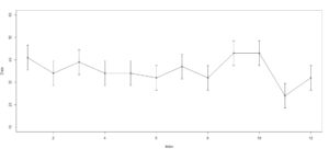
How to Plot the standard deviation of a dataset using R
You can plot the standard deviation of data using R by adding error bars to a plot. Here’s an example:
# set up standard deviation in R example
test <- c(41,34,39,34,34,32,37,32,43,43,24,32)

# Calculate the standard deviation using the sd() function
sd <- sd(test)

# Create a plot of the data using the plot() function
plot(test, type="o", ylim=c(10,60), ylab="Data")

# Add error bars to the plot using the arrows() function
arrows(x0=1:length(test), y0=test-sd, y1=test+sd, angle=90, code=3, length=0.05)
This example, using the base R plot function, generates the graph below.
Quickly Finding the Standard Deviation of a Data Set As a CSV File on The Web (or Your Computer)
Since the standard deviation is commonly calculated as an introductory descriptive statistic about a new data set, here’s an example of how to quickly hook up and calculate this kind of information for data in comma deiminated files (CSV files). In fact, you can even use this for CSV-formatted data files available on the web. The read.csv method in base R is just as happy to work with web-based data as read a file from your computer.
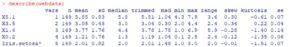
Here’s an example of downloading a web based CSV file (link to a broader tutorial that we wrote about using web based csv files), loading it into an R data frame, and generating the standard deviation for each of the fields in the data frame.
# use the read.csv method to read a web-based csv file, in this case the iris dataset
webdata <- read.csv("https://archive.ics.uci.edu/ml/machine-learning-databases/iris/iris.data")


# let's take a peek at the data using head()

> head(webdata)
  X5.1 X3.5 X1.4 X0.2 Iris.setosa
1  4.9  3.0  1.4  0.2 Iris-setosa
2  4.7  3.2  1.3  0.2 Iris-setosa
3  4.6  3.1  1.5  0.2 Iris-setosa
4  5.0  3.6  1.4  0.2 Iris-setosa
5  5.4  3.9  1.7  0.4 Iris-setosa
6  4.6  3.4  1.4  0.3 Iris-setosa

# continuing onwards, we use the sapply approach in base R to get standard deviation
sapply(webdata, sd)
This yields the following view…

Expanding on this a bit, here’s what you would generate if you used the describe () function in the psych library.
Interpreting Results
A low standard deviation relative to the mean value of a sample means the observations are tightly clustered. Larger values indicates that many observation(s) lie distant from the sample mean. This metric has many practical applications in statistics, ranging from measuring the risk of an error in hypothesis testing to identifying the confidence interval of a forecast or pricing the risk of an event in finance or insurance. Many data science and statistical learning algorithms incorporate some form of the standard deviation for automated screening & analysis. This measure also plays a key role in analyzing the results of a linear regression procedure. While the metric is broadly applicable, there is an underlying assumption the data values were generated by a random variable from the normal distribution if you intend to use the statistic for risk estimation or quantitative analysis.
As noted above, the sd() function uses the standard deviation formula for sample variance. If you are going to calculate the population standard deviation parameter, you will need to make the appropriate adjustment. The metric is sensitive to sample size, which has implications if you are watching the results of a repeated sampling process.
As you embark on a career as a data scientist or machine learning expert, you’ll discover that many of our core approaches are build around the concept of analyzing and optimizing the variance of a forecast’s errors, often measured using the standard deviation function. For example, linear regression – the core of classical statistics – is built around fitting a line to minimize the variance of the forecast error, giving more weight to extreme values (to whit, consider the concept of the mean squared error – your error measurements will quadruple every time your raw distance from the mean doubles). This approximates the expectations of real world humans. We can accept being slightly wrong on the details of a forecast, it’s the large gaps which will torpedo your credibility.
Need to work with standard error? We’ve got you covered here….
Related Materials