We have learned quite a bit of linear modeling through lm() function and delved into the world of stepwise linear regression. However, sometimes there is an issue of multicollinearity in the data. So, what is it? Multicollinearity in a dataset results when two or more predictors are highly correlated that they are unable to provide a meaningful and yet, independent insight of the regression model. Here, the Variable Inflation Factor (VIF) aids in determining the degree to which predictors are correlated to one another. So, how does it analyze it?
VIF takes into account the standard error aka the noise in the data along which the variance in each of the predictors. Another factor is the sample size which also determines the standard error and in turns the VIF. And lastly, the correlation of the predictors is another important aspect that should be considered.
You might be wondering, how VIF is interpreted? As a general rule of thumb, VIF values of 5 and above are concerning. However, we will explore it further as we move towards the examples. In this article, we are going to consider the “mtcars” dataset and take into account results from stepwise regression tutorial. Let’s kick off!
Doing the Pre-Requisites
We are going to use the same libraries that we have used in our previous tutorial on stepwise regression:
# Install Packages
install.packages(“tidyverse”)
install.packages(“caret”)
install.packages(“leaps”)
library(tidyverse)
library(caret)
library(leaps)
Creating the Model:
Just for a refresher, we have attained following equation from the previous tutorial of stepwise linear regression:
We are going to check if any of these predictors can cause multicollinearity. Let’s create a model and take a look at the summary statistics.
#Creating linear model and diplaying summary statistics
model <- lm(mpg~wt+qsec+am, data=mtcars)
summary(model)
Following summary statistics is displayed:
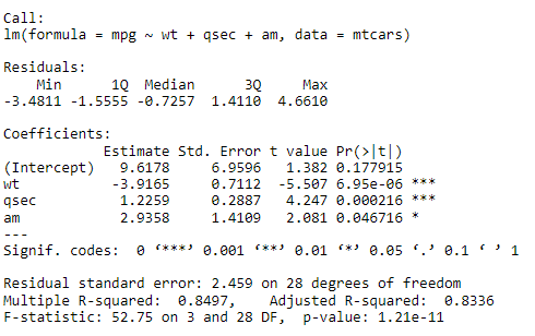
As you can see, the model’s estimated coefficients checks out with our linear model equation. Let’s move ahead and invoke the vif() function.
Finding the VIF
Prior to finding VIF, we are going to install “car” package and then invoke the VIF function.
# Using VIF function
install.packages(“car”)
library(car)
vif(model)
Following result is displayed:
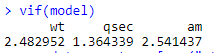
Well, none of the values are greater than 5. Let’s create another model that might have an issue of multicollinearity.
Exploring Another Model
At this moment, we are going to explore another model having disp, hp, wt, drat as the predictors.
#Another Model
new_model <- lm(mpg~disp+hp+wt+drat, data=mtcars)
summary(new_model)
Following output is displayed for the summary statistics:
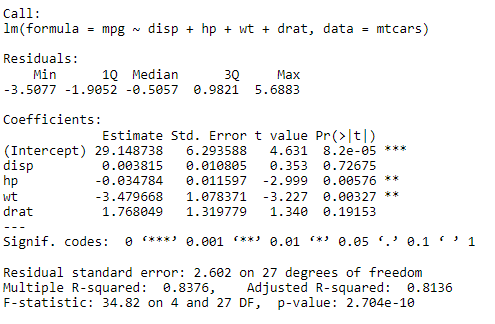
Everything looks great! Now, with this new model, let’s explore the VIF of it.
#Finding VIF of New Model
vif(new_model)
Output:
![]()
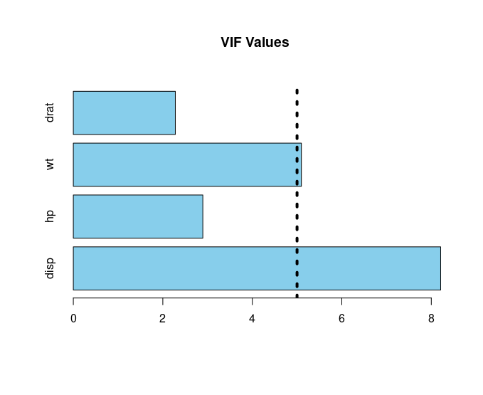
Here, it is evident that disp and wt predictors have VIF above 5.
Visualizing the VIF Values
We are going to use a horizontal barplot to visualize the result:
#Visualizing the Result
vif_values <- vif(new_model)
#Creating Horizontal Barplot
barplot(vif_values, main = “VIF Values”, horiz = TRUE, col = “skyblue”)
abline(v = 5, lwd = 4, lty = 3)
Output:
Concluding Remarks
With the VIF values determined, we are ready to embark on another journey of developing a correlation matrix which is covered in another tutorial. Nevertheless, it is evident that the predictors having VIF greater than 5 needs further treatment to make our model further refined.
Going Deeper!
If you’d like to know more, you can find it out here:
Linear Modeling
- How to Create Linear Model in R using lm Function
- Exploring the Predict Function in R
- Stepping into the World of Stepwise Linear Regression
Plotting: