How to Create a Linear Model in R using the lm Function

Linear regression is the cornerstone in predictive analytics and an essential tool for data science. In this article, we will explore different examples of using the ‘lm’ function in the R language and the significance of linear regression modeling as a whole. Linear modeling is of great help for data scientists who are striving for predicting an unknown variable values through one or more independent variables. So, how can you do it though R programming? Let’s embark on our linear regression journey.

As part of this article, we are going to use an inbuilt dataset in R called, “cars” which shows data points for cars’ speeds and the distances that they needed to stop. In order to fit the linear model in R, lm() function is used. Certainly there would be some pre-requisite steps.

Installing the Libraries

# installing the packages

install.packages(“tidyverse”)

install.packages(“modeldata”)

Next, you will have to load these libraries as well.

Loading the Libraries:

# loading libraries

library(“tidyverse”)

library(“modeldata”)

Now, load the builtin dataset “cars” with the following command:

# Choosing the Dataset

data(cars)

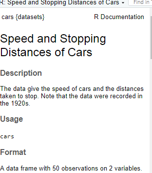
However, if you’d like to get a brief description of the dataset, you can type the following:

# Overview of Dataset

?cars

Following is the snippet of the output:

Taking a Peek at Data

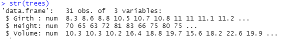
Once the dataset is loaded, another essential step is to check data integrity. Commonly used functions include str() and head(). Let’s use them and find out more about the data-types of each column.

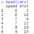
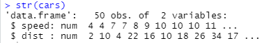
Based on the outputs, datatypes are consistent for analysis and we are good to go.

Watching lm() in Action

Prior to using lm() function for linear regression model, let’s look at the syntax of lm() function to get a better understanding of its syntax:

lm(<formula_for_fitting>,<dataframe>)

Based on the syntax it is essential for having a formula and a dataframe for the analysis:

# lm() in action

single.fit = lm(speed~dist, data=cars)

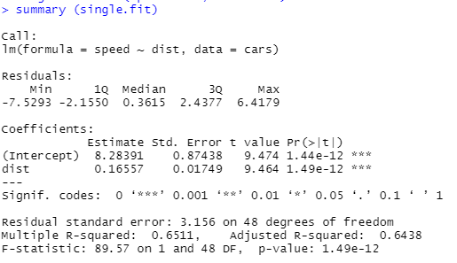
This store the linear model into the “single.fit” dataframe. Let’s explore the linear model through summary function

# Exploring lm() function

summary (single.fit)

Output:

Let’s visualize it through ggplot. However, first we need to invoke ggplot2 library:

#Creating a Plot

ggplot(cars, aes(x = speed,

y = dist))+

geom_point()+

geom_smooth(method = “lm”, se = FALSE)

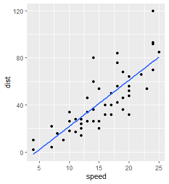
As evident from the plot, there is a strong positive correlation between stopping distance and speed of the cars which is also reflected from the summary() function.

Going forward with Multi-Variable Regression

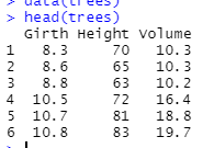
Let’s explore another dataset, “trees” which shows relationship between girth, height and volume of Black Cherry Trees.

#Accessing Another Dataset

data(“trees”)

Checking out the Data

Based on the data, let’s quickly check the data:

# Checking Data Integrity

head(trees)

str(trees)

glimpse(trees)

Output:

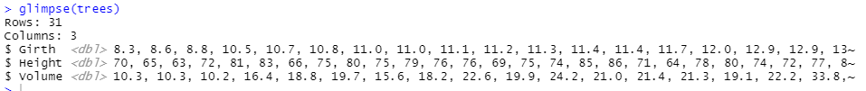
Once the data integrity is checked, let proceed towards multiple linear regression.

# lm() for multiple linear regression

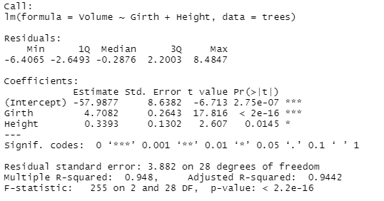
multi.fit = lm(Volume~Girth+Height, data=trees)

summary (multi.fit)

Following output would be displayed:

Concluding Remarks

Based on the outputs from lm() function, it is evident that correlation between different variables in a dataset can be explored in great depth using lm() function. The function can also serve as a foundation stone for creating models in which prediction of different values is also possible which will be covered in another article. For now, you might have a basic understanding of the single and multiple variable regressions as part of the activity.

Going Deeper…

If you’d like to know more, you can find it out here:

Linear Modeling:

Plotting: