Stepwise Regression, also known as, stepwise selection consists of a number of iterative steps that involves finding the most optimum model by adding or removing predictors from the subset of different variables. How should you do it? The key is AIC value along with other statistical signifance parameters that determines the suitability of the model. We will explore these terms as part of this tutorial. For starters, there are a total of three different stepwise regressions strategies; namely, forward, backward, and stepwise (sequential) selection. Here a brief overview of these key stepwise regression strategies:
- Forward Selection – It includes starting off with a no predictors and the predictors are kept adding on until an optimum model is reached.
- Backward (Elimination) Selection – It involves starting with all the predictors while removing the least collaborative predictors until all the predictors become statistically significant.
- Sequential (Both) Selection –It uses both forward and backward selection strategies. It begins with no predictors. Forward selection is performed in which a contributing predictor whereas in the next step the least contributing predictor is removed. This goes on till there is no improvement in statistical significance of the model.
So, we are going to explore a dataset “mtcars” which involves motor car road test trends while finding the best model through STEP() and STEPAIC() functions. At the end, we will compare the models obtained from different strategies. So, let’s get started!
Installing the Libraries
For stepwise linear regression, modeling a number of different libraries can be used; however, we will use the “caret” and “leaps” packages besides the “tidyverse” package. “Caret” package is quite useful for enhanced ease of machine learning capabilities whereas “leaps” is useful for stepwise regression calculations.
# Install Packages
install.packages(“tidyverse”)
install.packages(“caret”)
install.packages(“leaps”)
library(tidyverse)
library(caret)
library(leaps)
Invoking mtcars Dataset
In the next step, we are going to invoke the mtcars dataset
#Invoking Dataset
data(mtcars)
Stepwise Regression with STEP() Function
Before proceeding further, we will need to know the key variables needed for invoking STEP() function. Here is a simplified syntax of it:
STEP(<object>,<direction>,<scope>,<trace>)
For beginners, here is a brief overview of these arguments:
- An object is the linear model that can either be an intercept or a full linear model.
- The direction refers to the direction of stepwise regression
- The scope defines the formula that is considered as part of the step function
- Trace can avoid you the clutter by assigning it to FALSE or 0
we will have to install “statr” package as it will allow us to make regression analysis easier.
# Installing statsr packages
install.packages(“statsr”)
library(statsr)
Creating Intercept and Complete Models
Once, it is done let’s make two linear models that includes an intercept model that would serve as a null model for forward and sequential selection strategies along with a full model that will be suitable for backward selection.
# Creating the Intercept Model
intercept_only <- lm(mpg ~ 1, data = mtcars)
# Creating Complete Model
comp_model <- lm(mpg ~ ., data = mtcars)
Forward Selection with STEP() Function
In order to use STEP() function for the forward selection, we will use the following code:
# Doing Forward Stepwise Regression
for_reg <- step(intercept_only, direction=’forward’, scope=formula(comp_model), trace=FALSE)
To display the results of forward stepwise regression, we use:
#Results of Forward Stepwise Regression
for_reg$anova
Output:
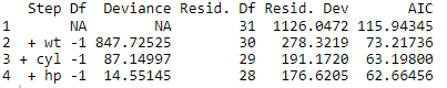
The output clearly shows the lowest AIC value that occurs while selecting three predictors. We can look for the final forward selection model as under:
# Final Forward Selection Model
for_reg$coefficients
Output:

Based on the output, following model can be made
Backward Selection with STEP() Function
We will follow the same steps with a few tweaks in code as under:
## Doing Backward Stepwise Regression
back_reg <- step(comp_model, direction=’backward’, scope=formula(comp_model), trace=FALSE)
Let’s get the results:
#Results of Forward Stepwise Regression
back_reg$anova
Output:
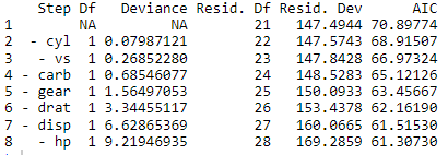
Based on the results, a total of seven predictors are eliminated. So, in order to the view the contributing predictors, we can type:
# Final Backward Selection Model
back_reg$coefficients
Output:

So, the backward selection model will be:
Sequential Selection with STEP() Function
For the sequential selection, we use the following code:
## Doing Sequential Selection Regression
both_reg <- step(intercept_only, direction=’both’, scope=formula(comp_model), trace=FALSE)
For the results, we use:
#Results of Forward Stepwise Regression
both_reg$anova
Output:
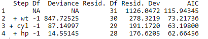
Here, three predictors are shown to be included in sequential selection. Let’s see how the final model looks like at the end.
# Final Sequential Selection Model
both_reg$coefficients
Output:

So, the sequential selection model would be:
By comparing the three model outputs, the forward and sequential selection models are identical whereas the backward (elimination) model is different. Let’s explore STEPAIC() function with sequential selection to get a better idea.
Sequential Stepwise Regression with STEPAIC() Function
Before proceeding with the full model creation, we will invoke MASS library as it will help us with choosing the best model based on AIC value.
## Stepwise Regression Using stepAIC()
library(MASS)
So, what is AIC? AIC stands for Akaike Information Criterion is estimator that can help us assess the model’s quality considering other models which makes it an important indicator for making the model selection quite easy.
For finding the best model through STEPAIC() let’s start off by the syntax:
STEPAIC(full_model, direction,trace)
Now, we will create a full-model through lm() function:
# Create the full model
full.model <- lm(mpg ~., data = mtcars)
In the next step, we will go with STEPAIC() function for each of the forward, backward, and sequential selections:
# Step AIC Both Selection
step_model_both <- stepAIC(full.model, direction = “forward”,
trace = FALSE)
summary(step_model_both)
Following output is displayed:
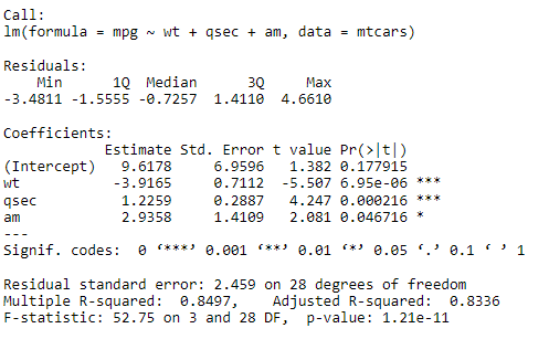
Based on the results, following model can be created through STEPAIC() forward selection:
Concluding Remarks
Based on the STEP() and STEPAIC() functions, the results for sequential selection model is identical. However, for finding the best model, we will have to compare the AIC of each model and find the one with the lowest. Out of the three models found using STEP() function, the one with lowest AIC of 61.307 is of backward elimination. Hence the best linear model would be:
Going Deeper…
If you’d like to know more, you can find it out here:
- How to Create Linear Model in R using lm Function
- Exploring the Predict Function in R