In this article we’ll get up and running on the Semantic Web in less than 5 minutes using SPARQL with R. We’ll begin with a brief introduction to the Semantic Web then cover some simple steps for downloading and analyzing government data via a SPARQL query with the SPARQL R package.
What is the Semantic Web?
To newcomers, the Semantic Web can sound mysterious and ominous. By most accounts, it’s the wave of the future, but it’s hard to pin down exactly what it is. This is in part because the Semantic Web has been evolving for some time but is just now beginning to take a recognizable shape (DuCharme 2011). Detailed definitions of the Semantic Web abound, but simply put, it is an attempt to structure the unstructured data on the Web and to formalize the standards that make that structure possible. In other words, it’s an attempt to create a data definition for the Web.
The primary method for accessing data made available on the Semantic Web is via SPARQL queries to a data provider’s endpoint. Endpoints are portals to data that a provider has made available for querying. This data is often published in RDF format. If you’re familiar with using SQL to query a database, then the idea of using a query language (SPARQL) to access a structured database or data repository (the endpoint) should be common ground. The practice is also similar to webscraping an XML document with a known structure.
The Semantic Web and R
A primary goal of the Semantic Web movement is to enable machines and applications to interface using standardized data definitions. As the Semantic Web grows, it will be ripe for mining with statistical programs that already lend themselves to automation – such as R. To that end, let’s dive into a simple query that will illustrate 75% of what you’ll be doing on the Semantic Web.
Accessing Data.gov datasets with SPARQL
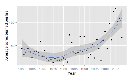
We’ll use data at the Data.gov endpoint for this example. Data.gov has a wide array of public data available, making this example generalizable to many other datasets. One of the key challenges of querying a Semantic Web resource is knowing what data is accessible. Sometimes the best way to find this out is to run a simple query with no filters that returns only a few results or to directly view the RDF. Fortunately, information on the data available via Data.gov has been cataloged on a wiki hosted by Rensselaer. We’ll use Dataset 1187 for this example. It’s simple and has interesting data – the total number of wildfires and acres burned per year, 1960-2008.
R code
Data.gov provides a Virtuoso endpoint, which we could use to submit manual queries. But we want to automate this process, so we’ll use Willem Robert van Hage and Tomi Kauppinen’s SPARQL package to access the endpoint.
library(SPARQL) # SPARQL querying package
library(ggplot2)

# Step 1 - Set up preliminaries and define query
# Define the data.gov endpoint
endpoint <- "http://services.data.gov/sparql"

# create query statement
query <-
"PREFIX  dgp1187: <http://data-gov.tw.rpi.edu/vocab/p/1187/>
SELECT ?ye ?fi ?ac
WHERE {
?s dgp1187:year ?ye .
?s dgp1187:fires ?fi .
?s dgp1187:acres ?ac .
}"

# Step 2 - Use SPARQL package to submit query and save results to a data frame
qd <- SPARQL(endpoint,query)
df <- qd$results

# Step 3 - Prep for graphing

# Numbers are usually returned as characters, so convert to numeric and create a
# variable for "average acres burned per fire"
str(df)
df <- as.data.frame(apply(df, 2, as.numeric))
str(df)

df$avgperfire <- df$ac/df$fi

# Step 4 - Plot some data
ggplot(df, aes(x=ye, y=avgperfire, group=1)) +
geom_point() +
stat_smooth() +
scale_x_continuous(breaks=seq(1960, 2008, 5)) +
xlab("Year") +
ylab("Average acres burned per fire")

ggplot(df, aes(x=ye, y=fi, group=1)) +
geom_point() +
stat_smooth() +
scale_x_continuous(breaks=seq(1960, 2008, 5)) +
xlab("Year") +
ylab("Number of fires")

ggplot(df, aes(x=ye, y=ac, group=1)) +
geom_point() +
stat_smooth() +
scale_x_continuous(breaks=seq(1960, 2008, 5)) +
xlab("Year") +
ylab("Acres burned")

# In less than 5 mins we have written code to download just
# the data we need and have an interesting result to explore!
If you’re familiar with R, the only foreign code is that in Steps 1 and 2. There we define the location of the endpoint and write the SPARQL query. If you have experience with SQL, you’ll notice that SPARQL syntax is very similar. The most notable exception is that Semantic Web data is structured around chunks of data that contain three pieces of information. In Semantic Web terminology these three pieces of information as referred to as subjects, predicates and objects and together they are called “triples”. A SPARQL query returns pieces of these chunks of data; exactly which pieces are returned depends on the query. We have defined a prefix which establishes that everywhere we say “dgp1187:” we want it to know that we mean “<http://data-gov.tw.rpi.edu/vocab/p/1187/>”. This saves us from having to retype long URIs every time we need to reference them. URIs are used extensively on the Semantic Web, so this is a very helpful feature.
In English, our query says, “Give me the values for the attributes “fires”, “acres” and “year” wherever they are defined, and assign them to variables named “fi”, “ac” and “ye” respectively. Also fetch the location of the value in the data as a variable called ?s and merge the other data values by that variable.”
The last bit of the query is the closest we get to SPARQL magic. Because the variable ?s is present in each clause of the query, our fire, acres burned, and year data will be merged by that variable. This is somewhat analogous to saying, “Once you’ve found a row of data that contains information on the number of fires, also return the acres burned and year data from that row and list them on the same row in the new dataset.” (If the logic behind the query isn’t yet clear, or you’re ready to see how you can make this query more advanced or parsimonious, the text and web pages in the “References” and “Additional Information” sections at the end of this article are good resources for learning SPARQL.)
Once defined, we pass this query and endpoint information to the SPARQL function which returns an object with two values – a data frame of the new data and a list of namespaces. At this point, we’re concerned with the data frame, so we pull it out in the last line of Step 2.
From that point on we treat the data just like any other dataset. Running some quick graphs, we see that although the number of fires per year have decreased, the number of acres burned per fire and the number of acres burned per year increased considerably between 1975 and 2008. (Despite being born in 1975, I disavow any responsibility for this trend.)
Summary
In a few short minutes, using R and SPARQL, we wrote code to pull and do initial analyses on an interesting government dataset. Hopefully, the power of R for mining the Semantic Web is evident from this simple example. As more data becomes available in RDF format, automated solutions for mining and analyzing the Semantic Web will become more and more useful.
Reference:
DuCharme, Bob (2011-07-14). Learning SPARQL . OReilly Media.
Additional Information:
Basic tutorial on querying Data.gov
More detailed tutorial on querying Data.gov
You may also be interested in our web scraping resources:
- Suggested Projects for Learning Web Scraping with R
- Importing CSV file data into R over the Web (a quick one liner)
- Using readlines() and RCurl for more advanced webscraping
- Scraping data into R from a JSON API
“http://services.data.gov/sparql” does not work as endpoint. I proved “https://www.data.gov/”. This url seems to provide xml code, but with errors. May it be that the endpoint url has changed?