Imagine if you could predict the future: Will there be a pandemic? Would there be an earthquake? On which day the stocks would rise? Who would win the next election?… One of the goals of data science is to process and analyze existing data so that we can forecast events to a certain degree of accuracy. Text analytics and text mining is a well established field of data science that aims to mine useful information from text data and incorporate that knowledge in various types of applications.
Raw data in the form of text is generated every second by all sorts of people in different ways such as forum comments, tweets, facebook updates, blogs, news, articles etc. There is a wealth of information out there, waiting to be mined and put to good use.
In this tutorial, I introduce you to some basic concepts of text mining using R language. R has a wide variety of packages available for building complex text mining applications. We’ll use the tidytext package for processing text and igraph and ggraph packages for visualizing it. Also, we’ll use the newsAPI to extract news articles from different sources and analyze them. I’ll show you how to visualize document hierarchy, generate word clouds and create document neighbor maps.
Using tidytext
The tidytext package was developed by Silge and Robinson and has some great facilities for manipulating and processing text. Let’s get our hands dirty and try out a few features. Start by installing tidytext by typing the following at R’s command prompt:
> install.packages(“tidytext") You’ll need the following libraries for this tutorial:
library(tidytext)
library(dplyr)
library(newsAPI)
library(SnowballC)
library(RColorBrewer)
library(wordcloud)
library(ggraph)
library(igraph)
The tidy data format has one token in one row. For now we’ll consider a word as a token. Lets do a simple example of cleaning text using gsub first. Later we’ll convert it to tidy format.
> txt <- c("First line of lines","It's a silver's lining of silver","123 of tree lines","in schools all lined up”)
> cleanTxt <- gsub(x=txt,pattern = "[0-9]+|'",replacement = "")
The gsub command above removes the numbers and quotation mark from text. The clean text looks like:
> cleanTxt
[1] "First line of lines"            "Its a silvers lining of silver"
[3] " of tree lines"                 "in schools all lined up"
Now let’s create a simple table using cleanTxt variable defined above:
> lines <- c(1,2,3,4)
> table <- tibble(text=cleanTxt,lines)
> table
# A tibble: 4 x 2
text                               lines
<chr>                              <dbl>
1 "First line of lines"                1
2 "Its a silvers lining of silver"     2
3 " of tree lines"                     3
4 "in schools all lined up"            4
The above table has 4 lines. We can convert it to tidy format using unnest_tokens() as shown below. Note that each row is a word/term:
> table %>% unnest_tokens(input=text,output=word) -> mytidyFormat
> mytidyFormat
# A tibble: 18 x 2
   lines word
   <dbl> <chr>
1     1 first
2     1 line
3     1 of
4     1 lines
5     2 its
6     2 a
7     2 silvers
8     2 lining
9     2 of
10    2 silver
11    3 of
12    3 tree
13    3 lines
14    4 in
15    4 schools
16    4 all
17    4 lined
18    4 up
Cleaning Text: Removing Stop Words and Stemming
You can think of raw text as “noisy” data. It has stop words, punctuations and different versions of the same word. Stop words are the commonly used words in text. Examples of stop words are: and, the, of, is, with etc. They are the basic building words for constructing sentences but may not convey useful information because of their abundance. Except for lines some special types of documents you would want to remove them from text. The package tidytext comes with a data set of stop words, which can be read into memory and then used to clean up the text. The following R code shows how you can remove stop words using anti_join.
> data("stop_words")
>  mytidyFormat %>% anti_join(stop_words) -> mytidyStopWordsRemoved

> mytidyStopWordsRemoved
# A tibble: 9 x 2
    lines word
    <dbl> <chr>
1     1 line
2     1 lines
3     2 silvers
4     2 lining
5     2 silver
6     3 tree
7     3 lines
Note how line, lining, lines, lined are all versions of the same word. To make them all consistent we can pass them through a process called word stemming, which removes the extra suffixes from the words to make them identical. Note that stemming changes a word to a consistent form but the resulting word may not have correct spelling. For example, virus is modified to “viru”, pandemic is changed to “pandem”, president becomes “presid”, etc. Let’s use the wordStem() function in R for the purpose of stemming.
> cleanStemmedText <- mytidyStopWordsRemoved %>%
                mutate(word = wordStem(mytidyStopWordsRemoved$word))
> cleanStemmedText
# A tibble: 9 x 2
    lines word
    <dbl> <chr>
1     1 line
2     1 line
3     2 silver
4     2 line
5     2 silver
6     3 tree
7     3 line
8     4 school
9     4 line
That looks great! We have cleaned up our text quite a bit. Now let’s move on to generating some interesting statistics.
Statistics From Text: TF, IDF, TF-IDF
We can use the count function to count the words in the cleanStemmedText as given below:
> cleanStemmedText %>% count(word)
# A tibble: 4 x 2
  word       n
   <chr>  <int>
1 line       5
2 school     1
3 silver     2
4 tree       1
From the point of view of text mining, it is good to have a word per document count. We can therefore use group_by and get counts w.r.t. a document or in the case of this simple example, we can count words per line as given below:
> cleanStemmedText %>%
     group_by(lines) %>%
     count(word) %>%
     ungroup()-> countTbl
> countTbl
# A tibble: 7 x 3
  lines word       n
   <dbl> <chr>   <int>
1     1 line       2
2     2 line       1
3     2 silver     2
4     3 line       1
5     3 tree       1
6     4 line       1
7     4 school     1
There are three most widely used statistical measures in text mining, i.e., term frequency (TF), inverse document frequency (IDF) and term frequency-inverse document frequency (TF-IDF). For anything and everything, I always advise to understand the math first, and then apply the concept (even if you have an awesome calculating platform like R to do it for you). So here goes an explanation in simple English:
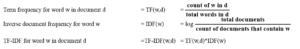
Note that IDF has only one parameter, i.e., word w with no dependency on document parameter d. This implies that IDF of a term is the same across all the documents. However, TF and TF-IDF of a word, vary depending upon a chosen count of w in d total words in d log total documents count of documents that contain w document. For our simple example, we are treating one line as an equivalent of a document. We can see that the word “silver” appears on line 2 twice. There are three total words in line 2, making TF(silver,2) = 2/3. Also, IDF(silver) = log(4/1) as there are a total of 4 documents and only one of them contains it.
The word “line” appears in every document and hence its IDF is log(4/4) = 0. Interesting! You can see why IDF is defined this way. Terms occurring in several documents lose their importance and have a lower IDF as compared to terms that occur only in a few documents. A term with a higher IDF, therefore, has more discriminating power between two documents as compared to the low scoring IDF terms (which are more commonly occurring terms). In many scenarios TF does not work well, so TF-IDF a combination of TF and IDF, is chosen to keep the balance between how frequently a term occurs in one document and how frequently it occurs across many documents. Let’s now generate TF, IDF, TF-IDF table in R as shown below:
> tfidfTbl <- bind_tf_idf(countTbl,word,document=lines,n)
> tfidfTbl
# A tibble: 7 x 6
  lines word     n    tf   idf tf_idf
  <dbl> <chr>  <int> <dbl> <dbl>  <dbl>
1     1 line       2 1      0     0
2     2 line       1 0.333  0     0
3     2 silver     2 0.667  1.39  0.924
4     3 line       1 0.5    0     0
5     3 tree       1 0.5    1.39  0.693
6     4 line       1 0.5    0     0
7     4 school     1 0.5    1.39  0.693
Wonderful! Now that we understand the nitty gritty details of TF-IDF, let’s go on to have some fun in R by extracting the news and analyzing it.
The NewsAPI
To extract news articles, I have chosen a very simple news API called NewsAPI. You can easily register and get an API key from there. The Github page describes how you can use the wrapper for R programming. Install this package by typing at the R command prompt:
> install.packages("devtools")
> devtools::install_github("mkearney/newsAPI")
Set the environment variable to use this API key and load the library:
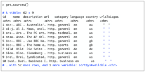
> sys.setenv("NEWSAPI_KEY" = “yourAPIKey") >library(newsAPI) You are good to go now. We’ll use two simple functions get_sources() and get_articles(). The function get_sources() returns the news source, its description and various other details. Below is the output from get_sources():
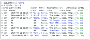
The get_articles command also returns a data frame. As input, it requires the name of the news source. Below is an example of articles retrieved from cnn news:
For the purpose of this tutorial we’ll use the following mapping:
Document: News source
Text: Title + description from all rows of the same news source
I like keeping the code modular so I have various functions to retrieve and clean the news text. In the box below is the code that retrieves news items from the internet:
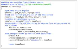
The first three lines of code with get_sources(), lapply() and do.call() are taken from here, which shows us how to get all articles in a bulk. We’ll make our own data frame called newsText that stores only the document (source of news e.g., bbc, cnn etc.), the text of the articles (title+description) and category (e.g., sports, technology, etc.). Output from this function is shown in the box below:
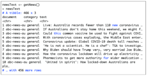
If you don’t want to use the news API right away to create this dataframe, I have saved this dataframe in a file called newsText.Rda.
You can type the following in R and use this data to reproduce the results shown in this tutorial:
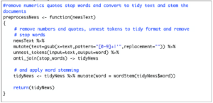
> load(“newsText.Rda") The next step is to pre-process the news and convert it to tidy format. The preprocessNews() function is given below. The code is self-explanatory:
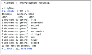
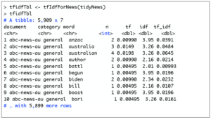
Let’s see what TidyNews looks like:
The last thing we need to extract are the statistics of words in each document. So here is a function to compute the tfidftable. We’ll make sure that we retain the category variable in the tfidftable by using the inner_join() function.
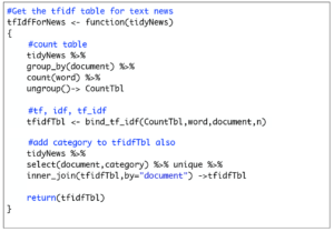
Here is what the TFIDF table looks like:
Displaying Hierarchy of Documents
Now that we have a word per row format as well as their corresponding statistics, we can start our analysis. When looking at text documents, it is always useful to understand the hierarchy of the documents. In R the igraph and ggraph libraries can be used to draw a dendrogram that shows the relationship of category with documents. Code below constructs a dataframe with “from” and “to” columns for creating an igraph object called g and generates a dendrogram using ggraph.
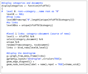
Let’s display the hierarchy of news documents by typing the following at the R prompt:
> displayCategories(tfidfTbl)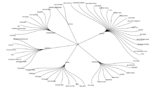
A very nice dendrogram is displayed. We can also consider the “general” category as the root and display the words having the higher scores for TF. You can play around with the following code and make your dendrograms for the other categories as well by using the “categ” argument of the displayGeneral() function.
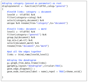
At the R command prompt type the following:
> displayGeneral(tfidfTbl) The following is displayed:
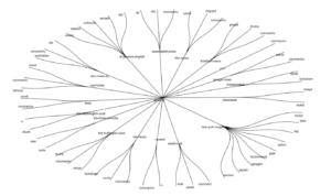
In case of ties in the highest TF scores, all words with ties are also displayed. Just displaying all these words with a high TF score gives us a rough idea of the contents of the documents. For example, you can see “coronaviru” (stemmed from coronavirus) in multiple documents. No surprise there, as we are right now living in the times of the pandemic!
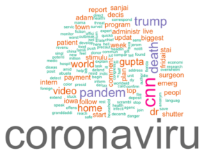
Displaying the Most Important Words
I like the idea of visualizing the most important words in a document using word clouds. Word clouds are the equivalent of plot, where the unit of data is a word. We’ll use the wordcloud() function, which requires a list of words and their corresponding frequencies. Let’s look at all the important words from the news source CNN. The box below shows how you can display all words with a TF greater than a certain threshold (used as a parameter):
#generate a word cloud for a particular document, when given the
#TF-IDF table and a threshold value
makeWordCloud <- function(tfIdfTable,doc="cnn",threshold=0.0001)
{
    tfIdfTable %>% filter(document == doc ) %>% filter(tf>threshold) -> doc
    wordcloud(doc$word,freq = doc$n*100,scale=c(4,0.1),
        colors = brewer.pal(8, "Dark2"))
}
Document Neighbors Map
One last thing that I would like to talk about is the document feature matrix, which is used commonly in text mining applications. In a document feature matrix, a row (say i) denotes a document and a column (say j) denotes a word. The (i,j) entry of the matrix can be count, TF or TF-IDF of the word in that document. The cast_dfm() function converts the tidy format to the document feature matrix easily. You can choose to include any feature of the word you like as a parameter to this function. If you place a binary 1 for a word present in the document and a 0 for a word not present in the document, then you get the popular bag of words representation. We’ll use the cast_dfm() function to add TF-IDF values in the matrix.
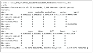
The dfm matrix is a sparse matrix, consisting mostly of zeroes. This is normal for text data as many words are not present in all documents combined. We can use dist() to compute a distance matrix between all pairs of documents using the dist() function. The closest neighbor of a document can then be visualized using ggraph library. The function below shows how you can do this:
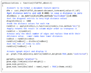
I have added comments in the code for getAssociations() to explain what each line is doing. The default value to the parameter nBest is set to one to indicate that only one closest document per row should be displayed in the graph but you can also set it to a different value. I am using Euclidean distance but you can use some other distance measure. Also, you can use correlation or another similarity metric to find the closest neighbor of a document. Of course, in that case, the closest neighbor would be the one having the highest similarity (rather than smallest distance). Calling this function in R shows the following graph:
> getAssociations(tfidfTbl)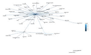
This gives us a nice map of documents close to each other w.r.t. Euclidean distance. Looks like there are many news sources that have Reuters as the closest document. We can also see a cluster of close documents that consists of news sources such as cnn, reddit-r-all, the-times-of-india, mtv-news, etc. Also, there is one isolated cluster of business-insider and business-insider-uk.
Further Readings
I hope you enjoyed this tutorial and found it useful for developing your own application. For an in depth study on this subject, you can refer to “Text Mining with R” by Silge and Robinson. It is available online and free. The authors demonstrate complex text processing, sentiment analysis and case studies using simple techniques and algorithms using the tidytext package. I thoroughly enjoyed reading this book.
About The Author
Mehreen Saeed is an academic and an independent researcher. I did my PhD in AI in 1999 from University of Bristol, worked in the industry for two years and then joined the academia. My last thirteen years were spent in teaching, learning and researching at FAST NUCES. My LinkedIn profile.