This tutorial is about a statistical test called the Shapiro-Wilk test that is used to check whether a random variable, when given its sample values, is normally distributed or not. In scientific words, we say that it is a “test of normality”. When I started writing this tutorial, I searched for the original paper by Shapiro and Wilk titled: “An analysis of variance test for normality (complete samples)”. It was published in 1965 and has more than 15000 citations. WOW! That’s awesome and they definitely deserve the title of “superstars of data science”. This goes on to show the importance and usefulness of the test proposed by them. Lets get down to the basics. First and foremost, let’s review the normal distribution.
The Normal Distribution
The normal distribution, also called the Gaussian distribution, is a favorite with the statistics and data science community. Without going into too many technical details, here is the expression for the probability density function of x when x is normally distributed:
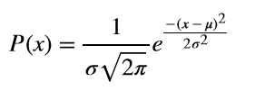
In the above expression is the mean and is the standard deviation of the distribution. If we set =0 and =1, then we have a special type of normal distribution called the standard normal distribution. If you look at the math expression closely, you can see that values away from the mean will have a small value of P(x) and values close to the mean will have a higher value. Moreover, because of the term, all values, which are equidistant from the mean, have the same value of P(x).
Let’s have some fun with R and look at what the shape of a normal distribution looks like.
Generating a Normally Distributed Variable in R
At the R console type:
> set.seed(19)
> x=rnorm(5000)
The set.seed(19) command sets the seed for the random number generator, so that the rnorm function generates the same random values every time you run it. Now you can exactly reproduce the results shown in this tutorial. rnorm(5000) will generate a vector with 5000 random values, all of which are sampled from a standard normal distribution (mean zero and standard deviation 1). Let’s visualize the frequency distribution by generating a histogram in R. Type the following at the console:
> hist(x,main = "Normal distribution")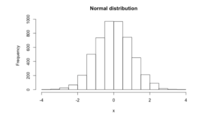
The histogram shows us that the values are symmetric about the mean value zero, more values occur close to the mean and as we move away from the mean, the number of values becomes less and less. This is in agreement with the P(x) expression we saw earlier.
Shapiro-Wilk Test
When the distribution of a real valued continuous random variable is unknown, it is convenient to assume that it is normally distributed. However, this may not always be true leading to incorrect results. To avert this problem, there is a statistical test by the name of Shapiro-Wilk Test that gives us an idea whether a given sample is normally distributed or not. The test works as follows:
Specify the null hypothesis and the alternative hypothesis as:
H0 : the sample is normally distributed
HA : the sample is not normally distributed
A test statistic is computed as follows:
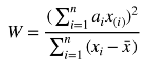
This W is also referred to as the Shapiro-Wilk statistic W (W for Wilk) and its range is 0<W 1. The lower bound on W is actually determined by the size of the sample. Normally distributed samples will result in a high value of W and samples deviating away from a normal distribution will have a lower value of W. Based on the value of W, we accept or reject the null hypothesis. Accepting the null hypothesis implies that we have sufficient evidence to claim that our data is normally distributed. Likewise, rejecting the null hypothesis in favor of the alternate hypothesis means that our data sample does not provide us sufficient evidence to claim that the sample is normally distributed.
In the expression, is the sample mean, x(i) is the ith smallest value in the given sample x (also called order statistic). ai are coefficients computed from the order statistics of the standard normal distribution. Let’s now apply this test in R.
Shapiro-Wilk Test in R
In R, the Shapiro-Wilk test can be applied to a vector whose length is in the range [3,5000]. At the R console, type:
> shapiro.test(x)You will see the following output:
Shapiro-Wilk normality test

data:  x
W = 0.99969, p-value = 0.671
The function shapiro.test(x) returns the name of data, W and p-value. Let us now talk about how to interpret this result.
P-values
When looking at the p-values, there are different guidelines on when to accept or reject the null hypothesis, (recall from our earlier.discussion that the null hypothesis states that the sample values are normally distributed). Generally we compare the p-value with a user defined level of significance denoted by alpha or a and make a decision as:
If p > a then accept H0
If p </= a then reject H0 in favor of HA.
The question remains on what should be the value of a . Depending upon your application you can choose a different significance level, e.g., 0.1, 0.05, 0.01 etc.. Michael Baron in his book: “Probability and Statistics for Computer Scientists” recommends choosing an alpha in the range [0.01, 0.1]. So for most applications you can safely accept H0 if p > 0.1 and safely reject H0 if p<0.01. For values of p in this range [0.01,0.1], it may be a good idea to collect more data if your application is a critical one. In the example above x is randomly sampled from a normal distribution and hence we get a p-value of 0.671 and we are sure to accept the null hypothesis that x is normally distributed.
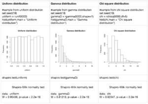
Shapiro-Wilk Test on Non-Normally Distributed Data
Let us now run some experiments and look at the p-values for different types of probability distributions which are not normal. The code for each experiment along with the histogram of the distribution and the result for the Shapiro-Wilk test is shown. For all the distributions given below we expect the p-value to be less than 0.01, which is exactly the case, so we can reject the null hypothesis. The histograms also show that the distributions do not resemble the symmetric normal distribution that we saw above.
Application: Demonstration of Central Limit Theorem in R
As a final note, I would like to show you a very interesting illustration of the central limit theorem and how we can confirm it via Shapiro-Wilk test. The theorem in simple words states that under some assumptions, the sum of independent random variables tends to a normal distribution as the number of terms in the sum increases, regardless of the distribution of these individual variables. Lets check the statement by taking the sum of uniformly distributed random variables and perform Shapiro-Wilk test to check the normality of the sum. I am taking the sum of random variables from a uniform distribution but you can check it equivalently for other distributions or even a mix of different distribution.
At the R prompt type the following lines of code:
#illustration of central limit theorem
set.seed(19)
z = runif(5000) #generate a sample distributed normally
for (i in 1:10)
{
z = z+runif(5000) #add another uniformly distributed variable
t = shapiro.test(z)
pVals[i] = t$p.value
WVals[i] = t$statistic
}
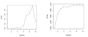
plot(c(1:10),pVals,type="b",xlab='Iteration')
plot(c(1:10),WVals,type="b",xlab='Iteration')The code generates z, a uniformly distributed random variable, next it adds another uniformly distributed random variable to it and performs the Shapiro-Wilk test, storing the p-values and W values after each addition. This is repeated 10 times. After the loop ends we plot the p-values and the W values on two different graphs.
The output pasted below is exactly what we expect. Initially, the p-values are very small, less than 0.01, leading to a rejection of the null hypothesis. As more and more variables are added to the sum our distribution of the sum tends to a normal distribution and hence we have p-values higher than 0.1, leading to an acceptance of the null hypothesis. The plot for W values also shows increasing W values as more random variables are added to the sum.
Further Readings
I hope you enjoyed this tutorial. You can download and read the original Shapiro and Wilks’ paper to understand the important properties of the test statistic W. It can be downloaded here.
About The Author
Mehreen Saeed is an academic and an independent researcher. I did my PhD in AI in 1999 from University of Bristol, worked in the industry for two years and then joined the academia. My last thirteen years were spent in teaching, learning and researching at FAST NUCES. My LinkedIn profile.