In this tutorial, I shall talk about one possible application of data mining, i.e., sentiment mining. The age of technology has built up a gold mine of data: social media, news feeds, blogs, discussion forums; many types of webpages are filled with lines and lines of text contributed by ordinary people from all walks of life. There is a wealth of information out there and we need to tap into this great resource.
Sentiment analysis is a specialized field of text mining, which can extract the subjective information from text and tell us about the moods, opinions, emotions and in general the sentiments reflected by a piece of text. Analysis of product reviews, posts and forums etc. offers endless possibilities: which product would most people buy? Which film would they watch twice? Are they satisfied by their present government? Which restaurant is the most popular? On which airline would they fly next? What is their next vacation spot? The list goes on and on. The ultimate aim of sentiment analysis is to answer such questions by analyzing the qualitative content of text data. There are many tasks involved in sentiment analysis. One of the key aims is to decide the polarity of text, which could be positive, negative or neutral. Another possibility is to mine emotions such as happy, sad, angry etc. or identify terms involving these emotions. In this tutorial, I will introduce you to the world of sentiment analysis and then we would go on to analyze J.K. Rolling’s spectacular book: Harry Potter and The Chamber of Secrets from the Harry Potter series.
An Overview of Sentiment Analysis
There are two most widely used methods for sentiment analysis: classifier based methods and lexicon based methods. In a classifier based approach, a dataset comprising text with labels (can be polarity, sentiment strength or emotions) is input to a machine learning algorithm, which in turn builds a model for classification. The learnt model is then used to predict the sentiments present in a given text sample. The second approach is the lexicon based approach, in which a dictionary of English words is maintained, each word having a corresponding sentiment label associated with it. This dictionary is also referred to as a sentiment lexicon. A given text sample is then classified based on an overall score of sentiments of the words comprising the sentence, where the individual scores are obtained via dictionary lookups.
You may wonder how this dictionary is built. Some sentiment lexicons are built manually by taking a list of words from the dictionary and getting many people (also called annotators) to labels these words with a sentiment and optionally also a sentiment score. Although, this is a very subjective approach but by having many annotators, a reliable and general dictionary of sentiment lexicons can be built. This then helps develop a very good general purpose application for sentiment analysis for a particular language. For a specialized and domain specific application you can use a classifier based approach.
The sentimentr Package in R
There are various possibilities for incorporating a sentiment analyzer in your application using R. I have chosen the sentimentr package by Tyler Rinker to demonstrate some important aspects of sentiment analysis. This package uses a lexicon based approach. The group of words in a sentence are then classified based on an overall score of sentiments of the words comprising the sentence. Let’s get down to the basics and see what sentimentr package can do for us. Start by installing the sentimentr package and loading its library.
library(devtools)
install_github(‘trinker/sentimentr’)
library(sentimentr)
Some other libraries that you need for this tutorial are given below:
library(dplyr)
library(RColorBrewer)
library(wordcloud)
Valence Shifters and Text Polarity
The great thing about the sentimentr package is that it incorporates valence shifters, which are words that alter the overall semantic meaning of a sentence. Rinker has explained valence shifters and how frequently they occur in text on his GitHub page. For example, for the word “happy” occurring in a sentence different valence shifters could be: negators (not happy), amplifiers (extremely happy), de-amplifiers (a bit happy) and adversative conjunction (was happy but the rain was a spoiler).
One of the basic functions that you can use is the sentiment() function. In the box below, I show you the command line and the output of this function:
> sentiment("I am excited")
element_id sentence_id word_count sentiment
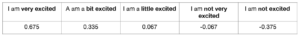
1: 1 1 3 0.4330127The sentiment() function returns a data frame with element_id, sentence_id, word_count and a sentiment score. It is important to look at the sentiment score in detail. A positive value indicates the strength of a positive sentiment and a value less than zero shows a negative sentiment. To have a better understanding of the sentiment score, we can try different versions of the word “excited”. I am pasting a summary below for different versions and their corresponding scores:
You can also use the same function to return the sentiments, sentence by sentence. Try the same function for multiple sentences. Pasted below is an example.
mytext <- c('I am happy and excited.  This is my first R application with sentiment scoring')
> sentiment(mytext)
element_id sentence_id word_count sentiment
1:    1           1          5    0.6708204
2:    1           2          9    0.0000000
The first sentence is certainly a positive sentiment and the second one is a neutral one. You can also try the sentiment_by() function that computes an overall polarity score for the entire text.
> sentiment_by(mytext)
element_id word_count     sd       ave_sentiment
1:    1         14     0.4743416     0.3660575
Another cool function in sentimentr package is the extract_sentiment_terms() function. This function returns the individual words along with their polarity strength and counts.
> t = extract_sentiment_terms(mytext)
> attributes(t)$count
       words   polarity n
1:       happy     0.75 1
2:     excited     0.75 1
3:           i     0.00 1
4:          am     0.00 1
5:         and     0.00 1
6:        this     0.00 1
7:          is     0.00 1
8:          my     0.00 1
9:       first     0.00 1
10:          r     0.00 1
11:application     0.00 1
12:       with     0.00 1
13:  sentiment     0.00 1
14:    scoring     0.00 1
Detecting Emotions
Let’s do a few more experiments. Instead of polarity of text, you may need to detect emotions. The emotion() function returns the rate of emotion per sentence. A data frame is returned by this function and of interest to us are the two columns: emotion type and emotion. Emotion indicates the strength of emotion present in the sentence.
Below, I am only pasting the output of the emotion() function for the first sentence. As the second sentence is a neutral sentence, all the emotion scores for it are zero.
> emotion(mytext)
element_id sentence_id        word_count     emotion_type emotion_count emotion
1:          1           1          5         anticipation             7     1.4
2:          1           1          5                  joy             7     1.4
3:          1           1          5             surprise             4     0.8
4:          1           1          5                trust             7     1.4
5:          1           1          5                anger             0     0.0
6:          1           1          5        anger_negated             0     0.0
7:          1           1          5 anticipation_negated             0     0.0
8:          1           1          5              disgust             0     0.0
9:          1           1          5      disgust_negated             0     0.0
10:         1           1          5                 fear             0     0.0
11:         1           1          5         fear_negated             0     0.0
12:         1           1          5          joy_negated             0     0.0
13:         1           1          5              sadness             0     0.0
14:         1           1          5      sadness_negated             0     0.0
15:         1           1          5     surprise_negated             0     0.0
16:         1           1          5        trust_negated             0     0.0
Similar to the sentiment_by() function, there is also an emotion_by() function that returns the average emotion of the entire text. I am pasting its output below as well.
> emotion_by(mytext)
element_id         emotion_type word_count emotion_count        sd   ave_emotion
1:          1         anticipation         14            7 0.9899495   0.5000000
2:          1                  joy         14            7 0.9899495   0.5000000
3:          1             surprise         14            4 0.5656854   0.2857143
4:          1                trust         14            7 0.9899495   0.5000000
5:          1                anger         14            0 0.0000000   0.0000000
6:          1        anger_negated         14            0 0.0000000   0.0000000
7:          1 anticipation_negated         14            0 0.0000000   0.0000000
8:          1              disgust         14            0 0.0000000   0.0000000
9:          1      disgust_negated         14            0 0.0000000   0.0000000
10:         1                 fear         14            0 0.0000000   0.0000000
11:         1         fear_negated          1            0 0.0000000   0.0000000
12:         1          joy_negated          1            0 0.0000000   0.0000000
13:         1              sadness          14           0 0.0000000   0.0000000
14:         1      sadness_negated          14           0 0.0000000   0.0000000
15:         1     surprise_negated          14           0 0.0000000   0.0000000
16:         1        trust_negated          14           0 0.0000000   0.0000000
Analyzing Harry Potter
Knowing the few basic commands in sentimentr package, we can now do some cool stuff. I have chosen Chamber of Secrets from Harry Potter book series as the raw text. You can install the “harrypotter” package using the following at the command prompt:
devtools::install_github(“bradleyboehmke/harrypotter") Let’s read the raw text of Chamber of secrets.
harry<-harrypotter::chamber_of_secrets Now using the sentiment() function, we can make a density plot to get an idea of the polarity of text.
#make a density plot of the sentiments present in text
makeDensityPlot <- function(txt)
{
    txt %>%
    get_sentences() %>%
    sentiment() %>%
    filter(sentiment!=0) -> senti

    densitySentiments <- density(senti$sentiment)

    plot(densitySentiments,main='Density of sentiments')
    polygon(densitySentiments,col='red')

return(densitySentiments)
}
If you have not seen the pipe operator %>% in R, I do suggest you get familiar with it and experiment with it. It is priceless. More information is available here. Briefly, this operator redirects the result of one operation to the next. So in the makeDensityPlot() function, txt is redirected to get_sentences, which in turn extracts the sentiments from text and redirects the output to filter out all the non-zero sentiments. The final output is stored in the variable senti. Next we use the density function to compute the kernel density of the sentiments in text.
Here is an example of how you call makeDensityPlot()
#uncomment if harrypotter package is not installed #devtools::install_github("bradleyboehmke/harrypotter")
library(harrypotter)
#read in chamber of secrets
harry<-harrypotter::chamber_of_secrets
makeDensityPlot(harry)
The final result looks something like this:
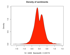
We can see that this density is multimodal with two peaks. There is one peak for negative sentiments and one peak for positive sentiments.
Making Word Clouds for Chamber of Secrets
Using the word cloud and the sentimentr package, we can make awesome wordclouds. Wordcloud is a graphical view of the most frequently used words in text. You can think of a wordcloud as the equivalent of a plot, with the difference that the unit of data is a word, rather than a number. We’ll use the wordcloud() function to generate a wordcloud. The function requires a list of words and their corresponding frequencies as a parameter. Extract_sentiment_terms() can be used to extract the words involving sentiments and instead of using their frequencies of occurrence, we can use the polarity of the word. Of course, you’ll have to multiply it by a large integer to make it look like a frequency. The following function can be used to visualize the words with positive or negative sentiments, depending upon the argument passed to it:
#for word clouds
#set pos to FALSE if negative sentiment words are to be displayed
makeWordCloud <- function(txt,pos=TRUE)
{
    terms = extract_sentiment_terms(get_sentences(txt))
    #get words with positive or negative polarity depending upon the argument
    if (pos)
    attributes(terms)$counts %>% filter(polarity>0) -> wordSummary
    else
    {  attributes(terms)$counts %>% filter(polarity<0) -> wordSummary
    #reverse the polarity for wordcloud
        wordSummary$polarity = wordSummary$polarity*-1
    }
    wordcloud(words=wordSummary$words,freq=wordSummary$polarity*100,
             max.words=250,colors = brewer.pal(8, "Dark2"), scale = c(1, 0.1))
}
In the code above polarity*100 is used for the frequency argument. The wordcloud() function displays the more frequently occurring terms in a bigger font compared to the less frequently occurring terms.
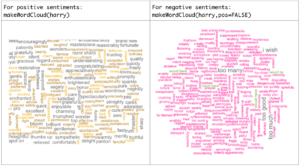
The figures below show the commands for displaying positive/negative sentiments and the corresponding wordcloud.
Plotting Emotions
The plot() function accompanied by the sentimentr package helps you visualize sentiments and emotions in text. You can plot a sentiment, sentiment_by, emotion or emotion_by object. Below, I show you an example of plotting an emotion_by object:
#plot the emotion_by object
plotEmotionBy <- function(txt)
{
    e<-emotion_by(get_sentences(txt),drop.unused.emotions=TRUE)
    plot(e)
}
You can call this function as follows:
plotEmotionBy(harry) The following is displayed:
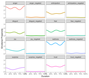
It is a nice plot if you want to look at the variation of individual emotions in a given piece of text.
Plotting Emotion Density in Chamber of Secrets
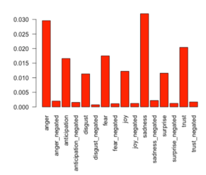
Instead of plotting individual emotions, it may be a good idea to extract the density of various emotions from text and then visualize them. A bar plot of all these emotions would give you a quantitative measure of how frequently an emotion occurs compared to the others. Paste the following function in R console or in your script file:
#make a barplot of different emotions
plotEmotions <- function(rawTxt)
{
    rawTxt %>%
    get_sentences() %>%
    emotion_by(drop.unused.emotions=TRUE) %>%
    group_by(emotion_type)  %>%
    summarise(ave_emotion=mean(ave_emotion)) -> txtSummary

    par(mar=c(11,4,4,4))
    barplot(txtSummary$ave_emotion,
         names.arg = txtSummary$emotion_type, las=2, col='red')
    return(txtSummary)
}
The above code is pretty neat as it is achieving a lots of things in just a few lines of code. The rawTxt argument is first broken up into sentences, which are in turn passed to emotion_by() function. The function returns various emotions, which are grouped by emotion_type and then summarized. This summary is then visualized using a bar plot. Enter the following command at the R console:
> plotEmotions(harry)The following bar plot is generated, where anger and sadness dominate all emotions:
Further Readings
I hope this tutorial inspires you into writing your own sentiment analysis application. For an in depth study on this subject, you can refer to “Text Mining with R” by Silge and Robinson. It is available online and free. The authors demonstrate complex sentiment analysis using simple techniques and algorithms, which heavily relies on the tidytext package.
About The Author
Mehreen Saeed is an academic and an independent researcher. I did my PhD in AI in 1999 from University of Bristol, worked in the industry for two years and then joined the academia. My last thirteen years were spent in teaching, learning and researching at FAST NUCES. My LinkedIn profile.