Someone who works a lot with data is definitely normalizing data on a very regular basis and if you plan to head into such a field, this is something you just cannot proceed without. The reason we need to normalize data in R is that data isn’t always neat and tidy; the way we’d want it to be for effective analysis. Different columns of our data may have very different scales. And many machine learning and analytics algorithms are very sensitive to the distance between consecutive observations in the data. The gradient descent algorithm, for instance, can go very wrong (or difficult) if the data is not on one scale.
We need to bring our data to one scale for fixing this problem. Normalizing brings every observation in the data on a scale between 0 and 1 while maintaining the relative position of each observation in the data frame, we therefore normalize data in R whenever the scales in our data do not match.
The Data
In this data normalization method, I’ll be using a built-in dataset of R called ‘cars’. It contains information about the speed and stopping distance (after the break was applied) for 50 different cars. We’ll begin by loading the dataset.
> data(cars)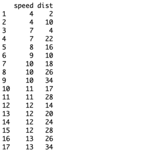
Before I normalize this data, I want to take some more time to emphasize on the importance of normalizing data. For that, let’s look at our data a little more closely.
> range (cars$speed)
[1]  4 25
> range (cars$dist)
[1]   2 120
You can see that the range (the smallest and the biggest observation) of speed is very different from the range of stopping distances. Therefore, a number of analytics algorithms wouldn’t be fully correct when run on this original data in raw form, this is because the distance between observations in the two columns are very different- data transformation, in this case a data normalization technique, is necessary to correct the feature scaling. As a solution, we will be normalizing this data to bring it into one scale, i.e., between 0 and 1.
Normalizing the Data
The formula for normalizing is given below.
Normalized Value = (Value – Minimum Value) / (Maximum Value – Minimum Value)
Here, the maximum value and minimum value refer to the largest and smallest values in the column we are working with. All there’s left to do is to apply this formula on every value in each column of the data separately. R gives you many ways for doing this, in the most basic sense, one would be using loops to traverse through every value of the data set and applying this formula. However, R makes that unnecessary, it manages the traversals on its own, you just need to specify an operation. Let’s proceed with an example of how this can be implemented.
> Normalize_Data <- function(val) { return ((val - min(val)) / (max(val) - min(val))) }The way I have defined my normalizing function is that it takes in an entire column of data and returns a column after traversing over every value and normalizing it. Here you may have noticed that there is no looping and R handles that bit on its own. This is one of the reasons that R has made data analytics fairly easy relative to low level languages.
With our function defined, we are ready to input values into it. I will now be storing the two columns of my data set i.e., speed and stopping distance into two variables which will be passed as arguments to the normalizing function. The returned columns of the function will be stored in the same variables.
> col_1 <- cars$speed
> col_2 <- cars$dist
> col_1 <- Normalize_Data(col_1)
> col_2 <- Normalize_Data(col_2)
In the above code, the variables ‘col_1’ and ‘col_2’ store the normalized columns of speed and stopping distance respectively.
> col_1
 [1] 0.0000000 0.0000000 0.1428571 0.1428571 0.1904762 0.2380952 0.2857143
 [8] 0.2857143 0.2857143 0.3333333 0.3333333 0.3809524 0.3809524 0.3809524
[15] 0.3809524 0.4285714 0.4285714 0.4285714 0.4285714 0.4761905 0.4761905
[22] 0.4761905 0.4761905 0.5238095 0.5238095 0.5238095 0.5714286 0.5714286
[29] 0.6190476 0.6190476 0.6190476 0.6666667 0.6666667 0.6666667 0.6666667
[36] 0.7142857 0.7142857 0.7142857 0.7619048 0.7619048 0.7619048 0.7619048
[43] 0.7619048 0.8571429 0.9047619 0.9523810 0.9523810 0.9523810 0.9523810
[50] 1.0000000
You can therefore see that all observations of speed have been scaled between 0 and 1. A similar result has been achieved for all the observations of stopping distance as well.
The Effect of Normalizing Data
Now that you have seen how I normalized the data for speed and stopping distance of the cars, we’ll spend a couple of minutes to understand the effect this had on our data. Remember that normalizing only brings all the variables in our data set on the same scale, it does not change the relationship of one variable with another and neither does it affect the distribution of the variable. Let’s try to verify this claim.
I’ll first plot the raw data and then the normalized data using a histogram, this should allow us to compare the distribution of both data sets.
> hist(cars$speed, main= 'Raw Speed Histogram')
> hist(col_1, main= 'Normalized Speed Histogram')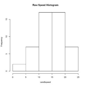
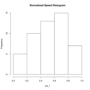
You can clearly observe and verify that the distribution of our normalized data and raw data is exactly the same, therefore, normalizing does not affect the relative position of an observation in a data set.
Moreover, we’ll now verify that the relationship of one variable with another is not changed by normalizing the data set.
> plot (cars$speed, cars$dist, main= 'Raw Data')
> plot (col_1, col_2, main= 'Normalized Data')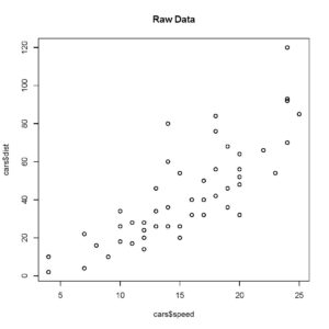
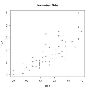
[You can therefore verify that the speed and stopping distance relationship is not altered by scaling the data between 0 and 1.
Normalizing data is a practice very commonly used by statisticians and machine learning engineers when working with data that uses many different variables that lie on different scales. If you are headed into the field, I highly encourage you to explore other ways to do this as well. R gives you many ways to go about a task and as a programmer, it is good to always find the most efficient method.