Introduction
Correlation is one of the essentials in the toolkit of a data analyst. The goal of correlation analysis is to determine, between two continuous variables, whether a change in magnitude and direction in one variable is associated with the other. This association (or non-association) is evaluated by a dimensionless decimal test statistic ranging from -1 to +1, generally called the correlation statistic / value. The closer a correlation value is to +1, the more positively correlated the two variables. Conversely, the closer it is to -1, the more negatively correlated the two variables are. And when the value is 0 (or close to 0), there is no correlation between the two variables.
Arguably the most common correlation analysis is the Pearson product moment correlation. It was developed by Karl Pearson, who is widely regarded as the father of modern statistics (Norton 1978). The pearson product moment correlation coefficient is denoted by the variable, r. Like all statistical methods, the pearson correlation comes with a set of assumptions.
Assumptions of the Pearson product moment correlation
There are more or less five assumptions to the Pearson correlation. To contextualize these assumptions, we shall use the built-in cars data set. This is a paired data set recorded in the 1920s of the speed of cars and the distances taken to stop.
data(“cars”)
str(cars)
## ‘data.frame’: 50 obs. of 2 variables:
## $ speed: num 4 4 7 7 8 9 10 10 10 11 …
## $ dist : num 2 10 4 22 16 10 18 26 34 17 …
1. Continuous variables
Both variables being compared must by of continuous data types. For ordinal data, other correlation methods like the Spearman’s rank-order correlation or the Kendall Tau correlation will be more appropriate.
A neat way to check whether the data in the data set it continuous is through the summary function. This gives you some descriptive statistics of your data set. If the variable is of a continuous data type the summary function returns its mean, median, minimum, maximum, and Q1 and Q3 interquartile ranges
summary(cars)
## speed dist
## Min. : 4.0 Min. : 2.00
## 1st Qu.:12.0 1st Qu.: 26.00
## Median :15.0 Median : 36.00
## Mean :15.4 Mean : 42.98
## 3rd Qu.:19.0 3rd Qu.: 56.00
## Max. :25.0 Max. :120.00
2. Paired, linear data
For the pearson correlation algorithm to be correctly implemented, all data points must be paired. Any unpaired data in the data set must be deleted. This is a non-negotiable assumption for this statistical test. Unpaired data must be removed from the data set before analysis.
The str function can help verify if all the data points in your data set are paired. It displays the structure of the R object. You should be noting that both variables should have the same number of observations.
str(cars)
## ‘data.frame’: 50 obs. of 2 variables:
## $ speed: num 4 4 7 7 8 9 10 10 10 11 …
## $ dist : num 2 10 4 22 16 10 18 26 34 17 …
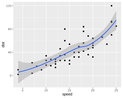
Morevoer, the paired data must have a linear association with each other (as opposed to having a polynomial relationship). A polynomial relationship implies that a line drawn over the regression may intersect it at more than one point. This implies that one level in the first variable is associated with multiple levels in the second.
Plotting the two continuous variables against each other using geom_point from ggplot2 and generating a regression curve using geom_smooth should allow you to determine whether the variables are linearly associated.
library(ggplot2)
ggplot(cars, aes(speed, dist))+
geom_point() +
geom_smooth(method = loess)
3. Independent of one another
Both variables must be measured independently of each other. One cannot be the factor of the other, nor be a derivative of the other. From the description of our data set, we can safely assume that there was a separate measuring device used for speed and for stopping distance.
4. Normally-distributed data
When Karl Pearson first discussed his correlation statistics, he suggested that the data must be normally distributed, this became a widely accepted unchallenged assumption. Interestingly, a study by Havlicek and Peterson (1977) suggests that the pearson $r$ is insensitive to extreme violation of the basic assumptions of normality and the type of measurement scale. Nefzger and Drasgow (1957) also suggest that the normality assumption is not necessary for the Pearson product moment correlation to be valid. These conclusions expand the application of the pearson correlation to a broader scope.
Nonetheless, most modern statistical references still recommend the normality assumption for Pearson correlation. And if the data is not normally-distributed, the Kendall Tau or the Spearman Rank is recommended.
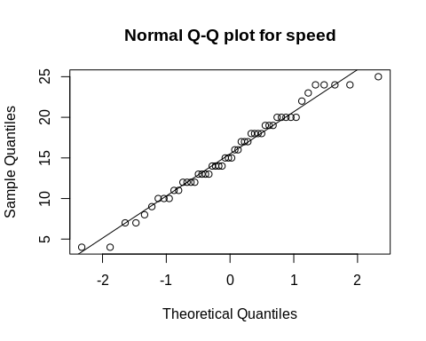
A quantile-quantile plot (Q-Q plot) is a good way to visualize normality. If the data points are distributed along the diagonal, then normal distribution is suggested.
qqnorm(cars$speed, main = “Normal Q-Q plot for speed”)
qqline(cars$speed)
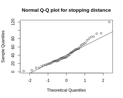
qqnorm(cars$dist, main = “Normal Q-Q plot for stopping distance”)
qqline(cars$dist)
Alternately, plotting a density plot using geom_density from the ggplot2 package should allow you to visualize normality and if not, the skewness of your data.
5. No extreme outliers
Potential outliers in the data can affect the pearson r. A good way to visualize outliers in a dataset is through a box plot. Potential outliers will reflect as points above (very high values) or below (very low values) the box plot. Here, I used the geom_boxplot from the ggplot2 to generate the box plots. The pivot_longer function from dplyr package makes it possible to display the box plots in one chart.
library(dplyr)
library(tidyr)
library(ggplot2)
cars %>%
pivot_longer(1:2, names_to = “var”, values_to = “value”) %>%
ggplot(aes(var, value)) +
geom_boxplot()
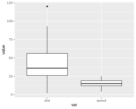
Based on the box plots, there is one outlier in the dist variable – the highest value. Since implementing the Pearson correlation in R is pretty straightforward, it should be best to perform the correlation with and without the potential outlier. And if both Pearson r values do not vary very much, then we can just leave that potential outlier in there.
But if you decide to remove that value, you must also remove its pair from the other variable. From the str output above, we see that the highest (max) value in the dist variable is 120. We can remove that value and its pair in the speed variable using the filter function from dplyr. We now have 49 data pairs.
cars.no.outlier <-
cars %>%
filter(dist != 120)
cars.no.outlier %>%
str()
## ‘data.frame’: 49 obs. of 2 variables:
## $ speed: num 4 4 7 7 8 9 10 10 10 11 …
## $ dist : num 2 10 4 22 16 10 18 26 34 17 …
Implementing the Pearson correlation
The cor function performs the pearson correlation by default. It can perform the Kendall Tau or the Spearman Rank if specified in the method argument. To implement the pearson correlation, you will extract the variables as vectors and call them in the cor function.
x <- cars.no.outlier$speed
y <- cars.no.outlier$dist
cor(x,y) # pearson is the default method. To use other correlation methods, input method = “kendall” or “spearman”.
## [1] 0.8046317
Alternately, you can convert the data frame into a matrix and call it in the cor function. This is particularly helpful if you have a data set where you want to correlate multiple variables with each other. The output will be a correlation matrix showing the pearson r for all combinations.
data.matrix <-
cars.no.outlier %>%
as.matrix()
cor(data.matrix)
## speed dist
## speed 1.0000000 0.8046317
## dist 0.8046317 1.0000000
Moreover, wrapping the cor function in a round function (e.g. round(cor(data.matrix), 3) will reduce the number of decimal places reported making the correlation matrix a little easy on the eyes. More information about the cor function can be found here.
The statistical significance of correlation coefficients are typically evaluated this way:
| Correlation coefficient | assessment |
| 1 | perfect positive correlation |
| 0.8 | fairly strong positive correlation |
| 0.6 | moderate positive correlation |
| 0 | no correlation |
| -0.6 | moderate negative correlation |
| -0,8 | fairly strong negative correlation |
| 1 | perfect negative correlation |
Thus given a pearson r of 0.805, we can conclude that there is a fairly strong positive correlation between the speed of cars in the 1920s and the distances it takes to stop.
Summary
The Pearson product moment correlation assumes continuous, paired data independently measured from each other, that is normally-distributed and free from extreme outliers. However, some studies suggest that the pearson correlation is not sensitive to violations of normality. But since, implementation of the Pearson (and as well as the Kendall and Spearman) is pretty straightforward in R, one can simply compare the different correlation values and find basis for their conclusion.
——
Havlicek, Larry L., and Nancy L. Peterson. 1977. “Effect of the Violation of Assumptions Upon Significance Levels of the Pearson r.” Psychological Bulletin 84 (2): 373–77. https://doi.org/10.1037/0033-2909.84.2.373.
Nefzger, M. D., and James Drasgow. 1957. “The Needless Assumption of Normality in Pearsons r.” American Psychologist 12 (10): 623–25. https://doi.org/10.1037/h0048216.
Norton, Bernard J. 1978. “Karl Pearson and Statistics: The Social Origins of Scientific Innovation.” Social Studies of Science 8 (1): 3–34. http://www.jstor.org/stable/284855.