R programming is one of the most enhanced statistical programming languages and provides extensive flexibility to estimate complex statistical properties for any academic and business domain. The libraries developed by the R community forum are the most significant ways to develop interactive web applications, analyse complex real-time financial data, prepare interactive visualization, and so on. So far, we have discussed how different R libraries can be used to solve real-world statistical problems. In the first part of this tutorial, we have calculated the consumer price index using dummy data set from the PriceIndices library. In this second part of the tutorial, we will also estimate the producer price index using the same library, but we will use producer data from Fred’s data server. In general, importing data sets into the R-Studio environment as a spreadsheet format is not complex, and we have already covered how to do that. In this tutorial, we will show you how to use the specific library to import data directly from Fred’s data server and then analyse the data set to calculate a combined producer price index. First, we will let you know how to use a specific library and get the needed information to pull producer data from Fred’s website directly to the R-Studio global environment. You can skip this step if you want, as you can also download a CSV file from Fred and then import the file into R-Studio by using the general file read function. Nevertheless, you want to sharpen your data analytics skills. In that case, we recommend you follow the step-by-step guideline of this tutorial to understand the data import, cleaning, and making a well-structured data frame to input in the producer’s price index calculation.
About the Tutorial:
In this tutorial we will use the following combination of price for a combined product price. Assume that we are trying to estimate a producer price index of peanuts.
Peanuts Production Cost = Packaging Cost (20%) + Peanuts cost (50%) + Freight cost (20%)
The company adds a 40% gross profit on the production cost and sell the final product. So the final selling price of the product is as follows,
Selling price = Peanuts Production Cost + 40% gross profit
Step-1
Install library
To start estimating the producer price index, we first need to collect the economic data, and we will use a specific library to pull out the required economic data from Fred’s data server. Let us open a new R script and run the following R code to install the required library.
install.packages(fredr)
install.packages(usethis)
After running the above-mentioned code, the two libraries will be installed in your R-Studio. As the library is installed, now you need to call the library by running the following code in your R-Studio console.
library(fredr)
library(usethis)
Get The API Key:
https://fred.stlouisfed.org/docs/api/api_key.html
If you have followed all the steps till now of this tutorial then you need to go to the official website of the Federal Reserve Bank of ST. LOUIS and sign up as a user. After your registration you can ask for an API key for R-Studio to import economic data directly to R-Studio for research purpose. Assuming you have got the API key and after that to connect the fred server to your R-studio you need to run the following code in your console.
fredr_set_key(“your API key”)
Step-2
Suppose you have successfully connected your R-studio to the data server. You can now follow the rest of this tutorial to learn how to estimate producers’ price indices using your selected economic data. In this tutorial, we will use three different producers’ data and clean it subsequently. You first need to import the selected data, and you can use the following R codes to do so.
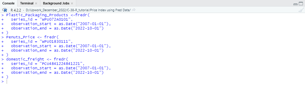
### Import Economic Data from Fred server ########
Plastic_Packaging_Products <-fredr(
series_id = “WPU072A0101”,
observation_start = as.Date(“2007-01-01”),
observation_end = as.Date(“2022-10-01”)
)
Penuts_Price <- fredr(
series_id = “WPU01830111”,
observation_start = as.Date(“2007-01-01”),
observation_end = as.Date(“2022-10-01”)
)
domestic_freight <- fredr(
series_id = “PCU4841224841221”,
observation_start = as.Date(“2007-01-01”),
observation_end = as.Date(“2022-10-01”)
)
Step-3
Check the Data set
Now that we have imported our specifically selected economic data from the server, it is time to check the properties of the data set and identify whether any corrections or adjustments are needed. Therefore, you need to have a general look at the overall data set, and by using the head function, you can quickly check the data set. Also, we will check if any missing values exist in the value column of our selected data set. You can quickly check the properties of the data set by running the following R code:
##### Check Properties of the Data set ######
head(Plastic_Packaging_Products )
is.na(Plastic_Packaging_Products$value)
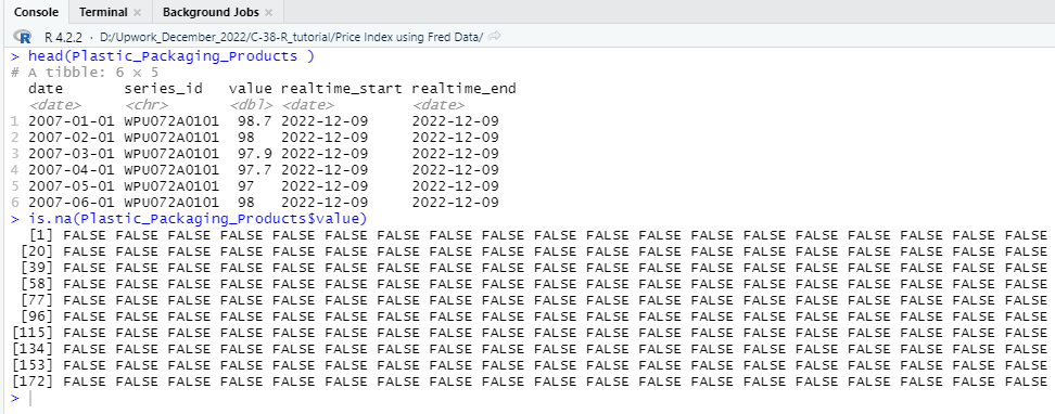
In the value column of one of the three data set does not contain any missing values and therefore we do not need to apply any measures for missing values. From now on we will clean our data set to make a combined data frame that will be suitable to use as input for price index calculation.
Step-4
The data set does not contain any missing value and therefore we can now clean the data sets to create a combine data frame. Here in this tutorial, we have selected three separate data set from fred and from the data set we only need the date and value column. Therefore, we only keep date and value column from each of the three data set previously imported as Plastic_Packaging_Products, Penuts_Price and domestic_freight. To do the cleaning first run the following R code in your R-studio console.
####### Data Cleaning #####
#### Plastic_Packaging ##########
Plastic_Packaging <- data.frame(Plastic_Packaging_Products$date,(Plastic_Packaging_Products$value*30)/100)
colnames(Plastic_Packaging)[1] = “time”
colnames(Plastic_Packaging)[2] = “prices”
df1 <- data.frame(Plastic_Packaging,
prodID = paste0(1))
head(df1)
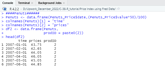
Here in the packaging data set we have calculated the cost of packaging by taking 30% of the total index price of Plastic Packaging. After that, we have named the date column as “time” and the calculated packaging cost as “prices”. After renaming the column, we have created a data frame using the two selected column and named the data frame a as df1. We will repeat the same procedure for PENUTS PRICE (50%) AND FREIGHT (20%). You just need to use the following codes to create the df2 and df3.
####Penuts Cost######
Penuts <- data.frame(Penuts_Price$date,(Penuts_Price$value*50)/100)
colnames(Penuts)[1] = “time”
colnames(Penuts)[2] = “prices”
df2 <- data.frame(Penuts,
prodID = paste0(2))
head(df2)
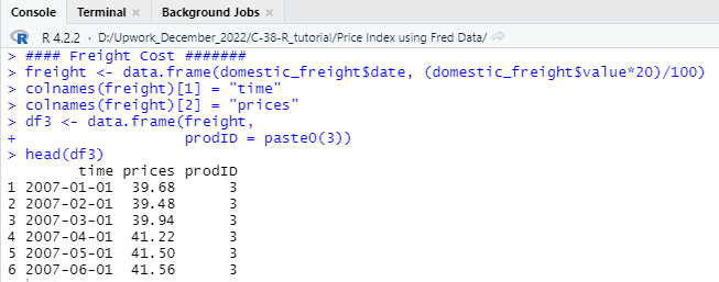
#### Freight Cost #######
freight <- data.frame(domestic_freight$date, (domestic_freight$value*20)/100)
colnames(freight)[1] = “time”
colnames(freight)[2] = “prices”
df3 <- data.frame(freight,
prodID = paste0(3))
head(df3)
Step-5
Now we will combine the df1, df2, and df3 so that we can calculate the total production cost. In the script we have created the All_cost variable and using that variable, we will calculate a 40% gross profit over the total production cost. So, to calculate the profit which we have set as df4 in the script, you need to run the following code first to combine the total cost.
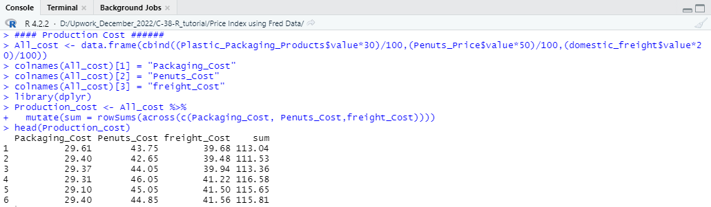
#### Production Cost ######
library(dplyr)
All_cost <- data.frame(cbind((Plastic_Packaging_Products$value*30)/100,(Penuts_Price$value*50)/100,(domestic_freight$value*20)/100))
colnames(All_cost)[1] = “Packaging_Cost”
colnames(All_cost)[2] = “Penuts_Cost”
colnames(All_cost)[3] = “freight_Cost”
library(dplyr)
Production_cost <- All_cost %>%
mutate(sum = rowSums(across(c(Packaging_Cost, Penuts_Cost,freight_Cost))))
head(Production_cost)
Step-6
We have combined the three data frame of product cost using the above-mentioned code and now we will calculate the 40% gross profit based on the total production cost of the product. The following R code will help you to calculate the profit and after that we will start creating the data set that will be required for price index calculation.
### Gross Profit Calculation ##########
profit <- data.frame(freight$time,(Production_cost$sum*40/100))
colnames(profit)[1] = “time”
colnames(profit)[2] = “prices”
df4 <- data.frame(profit,
prodID = paste0(4))
head(df4)
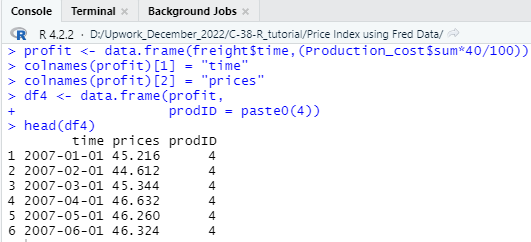
In the above code we have initially calculated the 40% gross profit from the total production cost and then created a data frame. The profit data frame then have been stored as a variable in the script as “profit”. Now as the profit data frame is created, we need to properly name the columns of the data frame so that all the column names of the different data frame is become same. To do that, we have named the Date column as “time” and the value column as “prices”. Apart from that, we also provided a category code of the profit data frame which is 4 and named the category column as “prodID”.
Step-7
In this section we will combine all the data frame which are df1, df2, df3, df4 based on the rows and to that we will use the rbind function. If you have followed all the steps till now, then you need to run the following code to bind the four data frame by rows.
############# Combining the 4 data frame #########
Combined_data <- rbind(df1,df2,df3,df4)
After combining the data frame, you will get a data frame as follows,
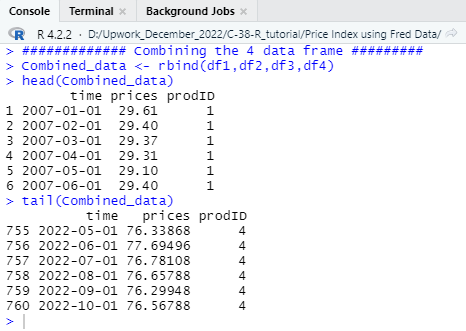
In all the four data frame there were three column which are “time”, “prices”, and “prodID” and those columns are added in the new data frame by rows. That means all the rows of df1 has placed first and then after the df1 and so on.
Step-8
In this step of the tutorial, we need to generate a quantity column in the combined data frame using random number generator. Note that, if you have a data set that already gave a quantity column then you do not need to use a hypothetical quantity column. As our selected data does not contain a quantity column therefore to make a data frame that can be inputted in the price index calculation, we must generate a quantity column. To generate a hypothetical quantity column in the combined data set, we have implemented the following r function.
quantity = list(sample(150 : 340, size = 760, replace = T))
head(quantity)
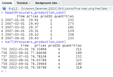
Procucers_production_cost <- cbind(Combined_data,quantity)
colnames(Procucers_production_cost)[4] = “quantities”
head(Procucers_production_cost)
We have used list function to generate a hypothetical quantity column to the combined data frame. In the random quantity we have selected size as 760 as the combined data frame consists of 760 rows also, we have set a range between 150 to 340 as the value of quantity so minimize the outlier from the data set. After generating the quantity column, we need to name the column as “quantities” as required for the price index calculation. So far, we have created a data frame as “Procucers_production_cost” and now we can apply functions of price index estimate easily.
Step-9
Final Producers Price Index Calculation:
From importing the data set from “fred” data server to the creation a combined data frame we have discussed a lot of things and if you carefully followed all the steps then you can now create the final index using the “PriceIndices” library of the R community. In the first part of the tutorial, we also discussed about how you can calculate a combined price index using sample data. In this second part of the tutorial, you have so far learned how to take raw data from a source and clean them to use in price index calculation. Now, as out data is well formatted and cleaned, we can run the following R code to calculate a combined Producers price index.
############ Index Calculation using Jevons method ###########
library(PriceIndices)
head(data_preparing(Procucers_production_cost, time=”time”,prices=”prices”,quantities=”quantities”))
jevons(Procucers_production_cost, start=”2007-02″, end=”2022-10″)
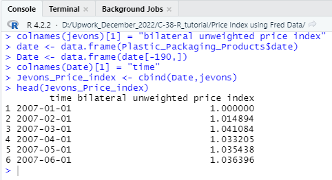
jevons <- data.frame(jevons(Procucers_production_cost, start=”2007-02″, end=”2022-10″, interval=TRUE))
colnames(jevons)[1] = “bilateral unweighted price index”
date <- data.frame(Plastic_Packaging_Products$date)
Date <- data.frame(date[-190,])
colnames(Date)[1] = “time”
Jevons_Price_index <- cbind(Date,jevons)
head(Jevons_Price_index)
If you successfully run the above code then you will get a combined bilateral unweighted producer’s price index using the Jevons method. The final index will look like as follows,
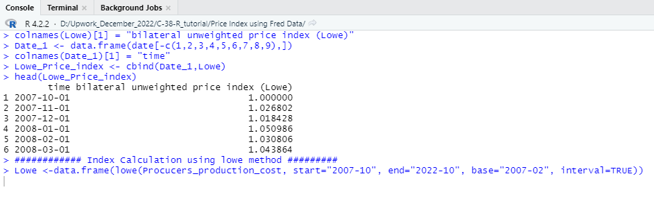
We will also use another price index calculation method named “Lowe” so that you can identify the difference in index values when we use different methods. By writing and running the following R code, you can easily calculate a “Lowe_Price_index”.
############ Index Calculation using lowe method #########
Lowe <-data.frame(lowe(Procucers_production_cost, start=”2007-10″, end=”2022-10″, base=”2007-02″, interval=TRUE))
colnames(Lowe)[1] = “bilateral unweighted price index (Lowe)”
Date_1 <- data.frame(date[-c(1,2,3,4,5,6,7,8,9),])
colnames(Date_1)[1] = “time”
Lowe_Price_index <- cbind(Date_1,Lowe)
head(Lowe_Price_index)
In this second part of the tutorial, we have discussed the Producers price index calculation wing R programming language in the most easiest way so that you can easily understand the entire process and implement the techniques to calculate Producer or consumer price index using any raw data. We have made this tutorial to provide you a clear understanding about the price index calculation and in upcoming days you will find more R programming tutorial like this which will help you to master your data analytics skills and implement them in your professional life.