Calculating a consumer price index is a great way to enhance your knowledge. The price index calculation is very advanced and complex when working with an extensive data set to create a consumer or producer price index. In general price index calculation is a process of using couple of variables related to the price index and combining them using empirically established statistical approach to formulate the final index. Suppose you learn the basics of processing extensive data using the R programming language and use innovative libraries to calculate the price index. In that case, you can deploy your skills to calculate any index related to economic growth, labour statistics, inflation rate, personal consumption expenditure, nominal GDP, and any economic variables.
Fundamentals of price index calculations:
When calculating price indices using the R programming language, you should first have gained basic R programming knowledge. Then you should carry forward your next project, where you will build a complete price index variable from massive data sets combined with numerous factors.
Calculating a price index using a small hypothetical data set may provide basic information about the whole process. Still, more than you will be required to learn to work with essential and fundamental world data sets. In this tutorial, we will discuss and build a price index model using the R programming language in R-Studio and discuss every possible topic necessary to follow while calculating a price index.
Step-1
You need to learn the basic information about the specific statistical package like “PriceIndicies.” The PriceIndices library is specially built to calculate the price index. It can handle extensive data sets to produce the final index. It would help if you remembered that this package contains functions requiring an advanced-capacity computer with good processing power and excellent graphics properties. Having a high-configuration laptop or desktop is essential to performing the complex tasks of this index calculation library, built with the R programming language.
Import or Install the PriceIndices package:
The first thing you need to do is import the PriceIndices package into your R-Studio environment. But, before that, if you still need to install the package, you need to install the library by running the following code in your R-Studio console.
Install.packages (“PriceIndices”)
You can also install the library manually from your R-Studio environment. To install the package manually you should follow the given steps.
- Click Tools → Install Packages
- Select Repository (CRAN) in the Install from: slot
- Type the package name (or several package names, separated with a white space or comma)
- Leave Install dependencies ticked as by default
- Click Install
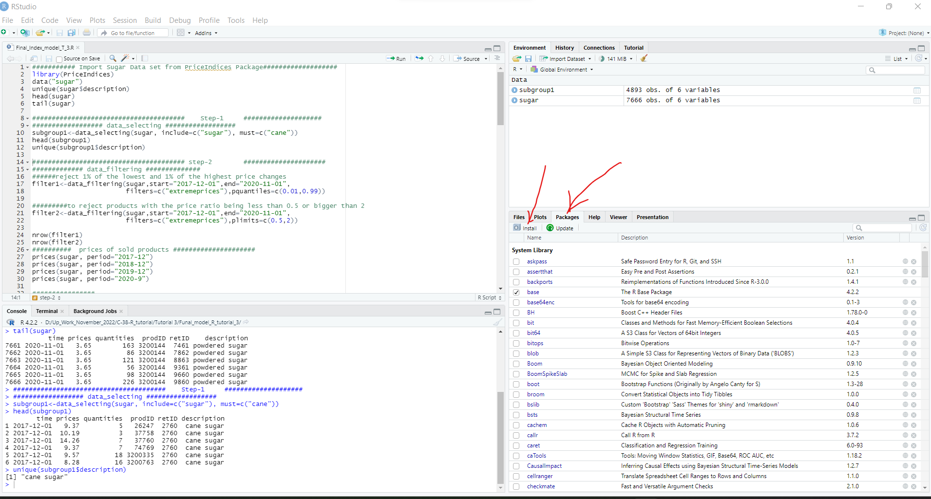
Figure-1: Install “PriceIndices” manually.
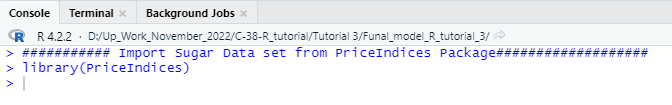
Now you need to import the library after installing it by running the following R codes in your R-Studio console.
library(PriceIndices)
Step-2
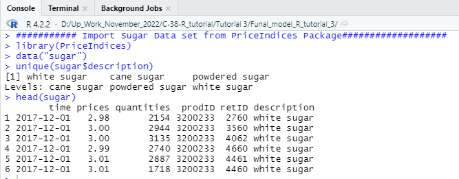
After installing the package, you can use a couple of built-in data sets to calculate your price index using the library. In this tutorial, we will use a sugar data set to build the final price index model. The first thing you need to do is import the data set in your R-studio environment and check the basic features of the data set. To import the data set and to evaluate the basic features, you can copy the following R code in your console and run it.
Code:
########### Import Sugar Data set from PriceIndices Package###################
library(PriceIndices)
data(“sugar”)
unique(sugar$description)
head(sugar)
tail(sugar)
**Notes: You should keep in mind that if you want to build price index for any custom data set then you need to arrange the data set according to the above mention format to carry on your calculation with the complex estimation of the PriceIndices packages.
Important Features of Sugar Data Set: The sugar data set contains six columns and from the given six columns retID column will not be necessary for the ongoing calculation but other five columns and its information’s are important for the price index calculation.
Step-3
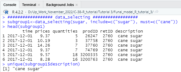
In this part of the tutorial, we will do some feature engineering to evaluate different properties of the data set. You can skip this process and jump into the index calculation but this step will teach you some very important features about how to create sub sets of the main data set and how to filter data using date time range. So, my honest recommendation for you is that you should also practice this step to deeply understand how the process works.
Code:
################## data_selecting ##################
subgroup1<-data_selecting(sugar, include=c(“sugar”), must=c(“cane”))
head(subgroup1)
unique(subgroup1$description)
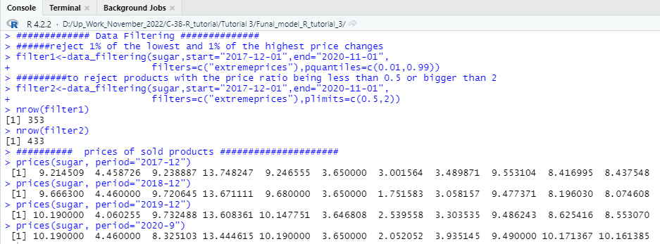
############# Data Filtering ##############
######reject 1% of the lowest and 1% of the highest price changes
filter1<-data_filtering(sugar,start=”2017-12-01″,end=”2020-11-01″,
filters=c(“extremeprices”),pquantiles=c(0.01,0.99))
#########to reject products with the price ratio being less than 0.5 or bigger than 2 #####
filter2<-data_filtering(sugar,start=”2017-12-01″,end=”2020-11-01″,
filters=c(“extremeprices”),plimits=c(0.5,2))
nrow(filter1)
nrow(filter2)
########## prices of sold products #####################
prices(sugar, period=”2017-12″)
prices(sugar, period=”2018-12″)
prices(sugar, period=”2019-12″)
prices(sugar, period=”2020-9″)
Step-4
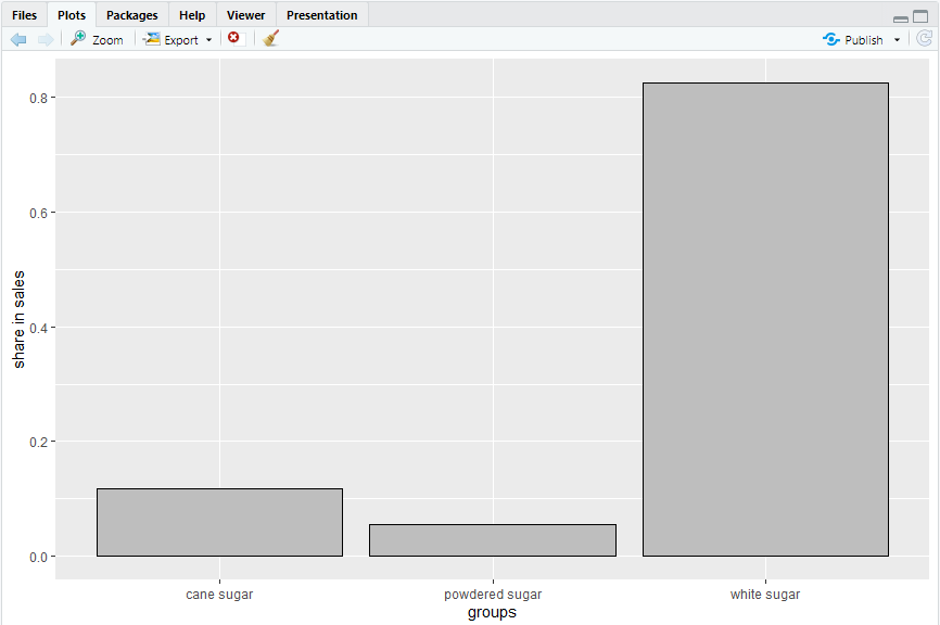
In this step, we will check the distribution of three different types of sugar in the data set and visualize them using a histogram. This visualization will help you understand the distribution of the three sugar types in the entire sugar data set. To create this visualization, you need to run the following R codes in your console and if you followed all the steps correctly, the following code would produce a histogram chart like the one given below.
Code:
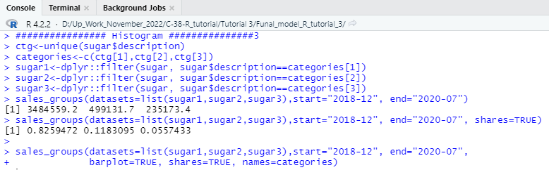
################ Histogram ###############3
ctg<-unique(sugar$description)
categories<-c(ctg[1],ctg[2],ctg[3])
sugar1<-dplyr::filter(sugar, sugar$description==categories[1])
sugar2<-dplyr::filter(sugar, sugar$description==categories[2])
sugar3<-dplyr::filter(sugar, sugar$description==categories[3])
sales_groups(datasets=list(sugar1,sugar2,sugar3),start=”2018-12″, end=”2020-07″)
sales_groups(datasets=list(sugar1,sugar2,sugar3),start=”2018-12″, end=”2020-07″, shares=TRUE)
sales_groups(datasets=list(sugar1,sugar2,sugar3),start=”2018-12″, end=”2020-07″,
barplot=TRUE, shares=TRUE, names=categories)
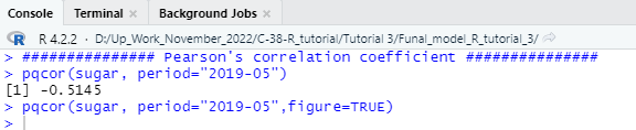
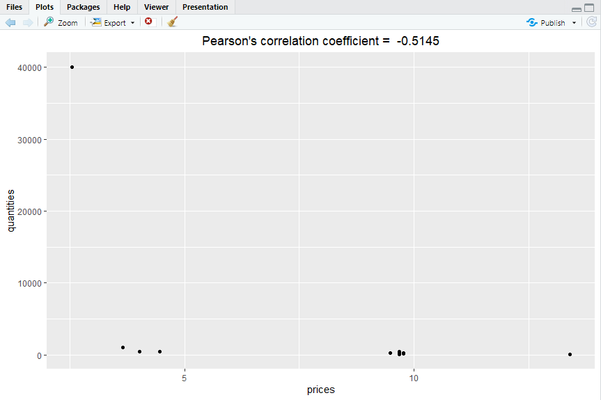
Now it is good to calculate the Pearson’s correlation coefficient value for the above-mentioned variables and deploy a scatter plot to check the relationship among variables. To calculate and visualize Pearson’s correlation coefficient you need to run the following code in your console to get the output.
Code:
############### Pearson’s correlation coefficient ###############
pqcor(sugar, period=”2019-05″)
pqcor(sugar, period=”2019-05″,figure=TRUE)
Step-5
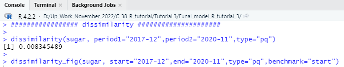
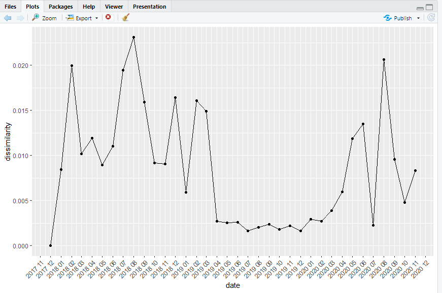
Now let’s check some important features of the examined variable in this tutorial. In this step we will check the dissimilarity value of the relative prices of sugar against different quantities over the selected time period. To calculate the dissimilarity value, we will use specific function from the PriceIndices package and also plot the result using a line chart that connects all the points over the time period. We have selected the time period from December 2017 to November 2020 which will be displayed in the X axis of the line plot.
Code:
################# dissimilarity #####################
dissimilarity(sugar, period1=”2017-12″,period2=”2020-11″,type=”pq”)
dissimilarity_fig(sugar, start=”2017-12″,end=”2020-11″,type=”pq”,benchmark=”start”)
Step-6
Bilateral unweighted price index calculation
Now, we have covered almost every necessary evaluation process we may check whenever we try to calculate a final price index using dummy data or even real-world data. From now on, we will use different methods and functions of the “PriceIndices” packages to calculate the price index. We will estimate this first index using the Jevons function. In this step, we must specify the date range, which means we must select a specific period for our index calculation. For example, if we want to calculate the consumer price index for the fiscal year 2022, then we need to select the year’s starting date and the year’s ending date. We have used December 2017 as the starting period for the price index and November 2020 as the index’s end. Following this process, if you run the following R code in your console, you will get a bilateral unweighted price index for the chosen sugar data set.
Code:
######## bilateral unweighted price index calculation ##################
jevons(sugar, start=”2017-12″, end=”2020-11″)
jevons(sugar, start=”2017-12″, end=”2020-11″, interval=TRUE)
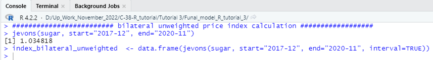
We have successfully calculated the bilateral unweighted price index using the sugar data set. You can rearrange the index in a data frame to easily display the calculated index and export the index in a spreadsheet format. To create the data frame, you need to follow the codes given below step by step.
Code:
#### Change Column Name ##########
colnames(index_bilateral_unweighted)[1] =”Unweighted_Price_Index”
head(index_bilateral_unweighted)
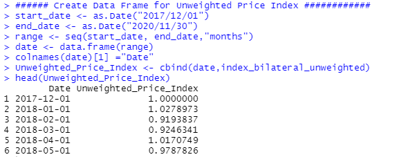
###### Create Data Frame for Unweighted Price Index ############
start_date <- as.Date(“2017/12/01”)
end_date <- as.Date(“2020/11/30″)
range <- seq(start_date, end_date,”months”)
date <- data.frame(range)
colnames(date)[1] =”Date”
Unweighted_Price_Index <- cbind(date,index_bilateral_unweighted)
head (Unweighted_Price_Index)
Step-7
So far, you have learned how to calculate different statistical measures of price index and have successfully calculated one price index. Now let us calculate another price index, which will be calculated using the lowe function from the PriceIndices packages. You can run the following codes in your R-Studio console to estimate the price index of this kind.
Code:
####### Lowe Price Index #############
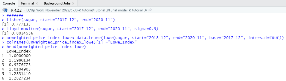
fisher (sugar, start=”2017-12″, end=”2020-11″)
lloyd_moulton(sugar, start=”2017-12″, end=”2020-11″, sigma=0.9)
unweighted_price_index_lowe<-data.frame(lowe(sugar, start=”2018-12″, end=”2020-11″, base=”2017-12″, interval=TRUE))
colnames(unweighted_price_index_lowe)[1] =”Lowe_Index”
head(unweighted_price_index_lowe)
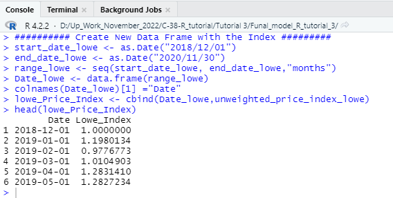
########## Create New Data Frame with the Index #########
start_date_lowe <- as.Date(“2018/12/01”)
end_date_lowe <- as.Date(“2020/11/30″)
range_lowe <- seq(start_date_lowe, end_date_lowe,”months”)
Date_lowe <- data.frame(range_lowe)
colnames(Date_lowe)[1] =”Date”
Date_lowe
lowe_Price_Index <- cbind(Date_lowe,unweighted_price_index_lowe)
head(lowe_Price_Index)
Step-8
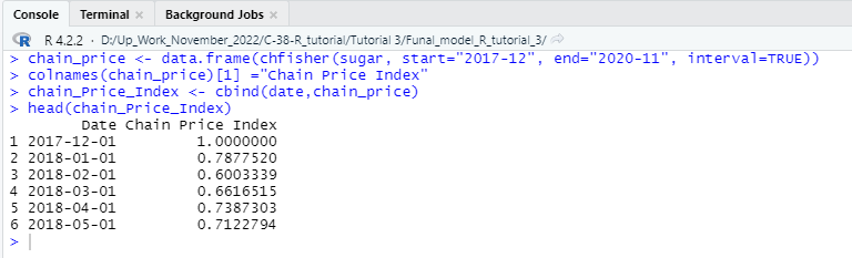
Let us calculate another type of price index that can be calculated using chfisher function from the following library.
Code:
############### chain price index calculation ########################
chain_price <- data.frame(chfisher(sugar, start=”2017-12″, end=”2020-11″, interval=TRUE))
colnames(chain_price)[1] =”Chain Price Index”
chain_Price_Index <- cbind(date,chain_price)
head(chain_Price_Index)
Step-9
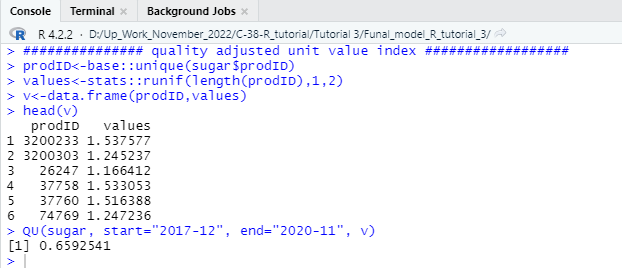
In this step of our consumer price index tutorial, we will learn how to estimate the quality-adjusted unit value and index using the QU function of the PriceIndices library. To estimate the quality-adjusted price index, you can run the following R codes in your R-Studio console.
Code:
############### quality adjusted unit value index ##################
prodID<-base::unique(sugar$prodID)
values<-stats::runif(length(prodID),1,2)
v<-data.frame(prodID,values)
head(v)
QU(sugar, start=”2017-12″, end=”2020-11″, v)
Step-10
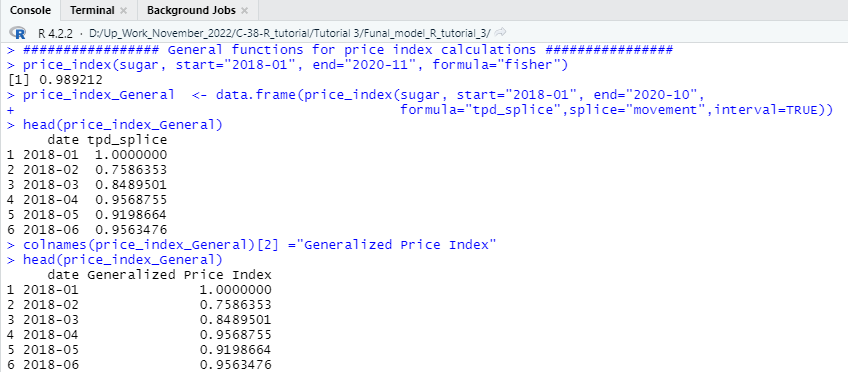
So far, we have learned to calculate several approaches through which we can estimate a standardized consumer price index using some unique functions and features of the PriceIndices library. We will learn to calculate the general price index and features using the R programming language. To calculate the generalized consumer price index for any standard consumer price data set, the following functions and procedures will benefit you. You can easily calculate the generalized consumer price index by customizing the following R code to the needs of your chosen data set.
Code:
################# General functions for price index calculations ################
price_index(sugar, start=”2018-01″, end=”2020-11″, formula=”fisher”)
price_index_General <- data.frame(price_index(sugar, start=”2018-01″, end=”2020-10″,
formula=”tpd_splice”,splice=”movement”,interval=TRUE))
colnames(price_index_General)[2] =”Generalized Price Index”
head(price_index_General)
Step-11
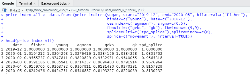
In step 10, you learned how to calculate a generalized consumer price index using only one (fisher) specific method of price index calculation. Now, as we are trying to estimate a finalized price index, it is wise to compare the results of the price index estimated by different methods. The comparison will tell us how the value of the price index differs when we use different approaches. The following will allow you to create a data frame showing the index value estimated using different statistical methods. We will create a function; we will specify the date range and also include a couple of different methods in one function to estimate the price index.
Code:
#### Different Methods of Price Index Estimation in One specific Pipeline function ########
price_index_All <- data.frame(price_indices(sugar, start=”2019-12″, end=”2020-08″, bilateral=c(“fisher”),
bindex=c(“young”), base=c(“2018-12”),
cesindex=c(“agmean”), sigma=c(0.5),
fbmulti=c(“geks”, “gk”), fbwindow=c(9,9),
splicemulti=c(“tpd_splice”),splicewindow=c(6),
splice=c(“movement”), interval=TRUE))
head(price_index_All)
Conclusion:
The index calculation is an advanced-level tutorial that requires proper knowledge and understanding of basic R programming and basic knowledge of statistics, mathematics, and economics. We have discussed it straightforwardly so that any learner can understand the estimation. Throughout the tutorial, we have discussed the basic procedures of consumer price index using a couple of different approaches from the PriceIndices library of the R-Studio. This article will provide essential to advanced working knowledge on using R programming language to import different data sets in the R-Studio environment, create basic graphs, construct data frames, and perform other necessary tasks.
We have covered the first part of the tutorial. If you successfully understand the entire tutorial, you can now work with an accurate world data set. We will soon come up with the second part of the tutorial, where we will use actual world data sets, clean them, make them usable for price index calculation, and finally estimate the price index using the data set.