The Kruskal Wallis test in R is a non-parametric method to test whether multiple groups are identically distributed or not. The word “non-parametric” implies that we do not have to make any assumptions about the underlying distribution of data. To explain this test, I have chosen a built in dataset in R called “chickwts”. I’ll illustrate the various steps involved in this test by using side by side examples of chickwts statistics.
Chickwts dataset Let’s first look at the chickwts dataset. You can type the following in R to get more details about the dataset:
>?chickwtsType chickwts at the R command prompt:
>chickwtsPasted below are the first 11 lines from an output of 71 lines.
   weight      feed
1     179 horsebean
2     160 horsebean
3     136 horsebean
4     227 horsebean
5     217 horsebean
6     168 horsebean
7     108 horsebean
8     124 horsebean
9     143 horsebean
10    140 horsebean
11    309   linseed
The dataset has two variables, i.e., “weight” and “feed”. “Feed” has various categories, which can be listed using the following command in R:
> levels(chickwts$feed)The output gives us the names of 6 different types of feed and is shown in the box below.
[1] "casein" "horsebean" "linseed" "meatmeal" "soybean" "sunflower"Visualize the dataset It is always a good idea to get familiar with the dataset or data frame before doing any experiments on it. If you like working with numbers, you can get a nice numeric summary of the data set using the “table” function. Type the following at the R console:
> table(chickwts$feed,cut(chickwts$weight,breaks=5)) (108,171] (171,234] (234,297] (297,360] (360,423]
casein 0 2 2 4 4
horsebean 7 3 0 0 0
linseed 3 4 4 1 0
meatmeal 1 1 4 4 1
soybean 2 3 6 3 0
sunflower 0 1 2 7 2The “breaks” in table function specifies 5 discrete ranges for weight. The numbers in the output table are the number of observations of each feed category (treatment groups) in that weight range.
Sometimes, you may want to visualize the data instead of looking at numeric summaries. I have written a small piece of code to plot the weight values for each category of feed in a different color on the same plot. Type the code below in R:
#Kruskal Wallis Test
totalLevels = length(levels(chickwts$feed))
#colors for different groups colorList=c("green","blue","red","yellow","orange","purple")
#initial dummy plot plot(1,xlim=c(1,totalLevels),ylim=range(chickwts$weight),col="white",
    xlab="feed",ylab="weights",xaxt="n")
j <- 1
for (i in levels(chickwts$feed))
{
    ind = chickwts$feed == i
    points(rep(j,sum(ind)),chickwts$weight[ind],col=colorList[j])
    j <- j+1 }
#label the x-axis
axis(1,at=1:6,labels=levels(chickwts$feed))
This creates the following plot:
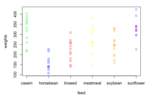
The problem with the above test data graph is that there are overlapping points with the same weight and hence do not convey much about the frequency of values in each category. We cannot really make out the median values of data and neither can we tell where the most frequently located values in the data are.
Instead of a scatter plot you can use a box plot, which is a well known method for visualizing categorical data. If you do not know about box plots you can see their details here. Box plots are easy to create in R using the “boxplot” command. You can use the “col” optional argument (specifies colors) for which I am using the colorList, defined earlier in our code.
> boxplot(weight~feed, data=chickwts, col=colorList)The argument weight~feed specifies that weight is the dependent variable and feed is the independent variable. The corresponding box plot is shown below:
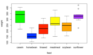
The box plot is a nice visualization of the various groups of chicken based on their feed. We can see a significant difference between various categories, e.g., casein vs. horsebean. The box plots also show us the median of data, the outliers and the general spread of data.
Kruskal Wallis Rank Test
In the chickwts dataset, there are 6 different categories of feed and we want to know if all feeds have the same effect on the growth rate of chickens. In technical words, we want to know if the “distribution of the weight” of chickens is the same for all types of feed or not. This is important as a significant difference would indicate that there is a category or multiple categories of feed, which may result in a lesser (or higher) than desired growth rate of chickens. It can, therefore, help make good informed decisions about the feed to use in a poultry farm. When we created the box plot we visually examined that the groups based on feed are quite different from each other, except a few pairs that look similar, e.g., linseed (red) and soybean (orange) groups look very similar, and casein (green) and horsebean (blue) look quite different. We can use Kruskal Wallis rank sum test to verify that at least one of the groups is different from the rest. Below are the three steps to carry out the Kruskal Wallis test:
Step 1: State the hypothesis
The first step in carrying out any statistical test is to formulate the null hypothesis H0 and the alternate hypothesis HA.
H0: All 6 groups of chicken feed are the same
HA: There is at least one group of chicken feed, which is different from the rest
Step 2: Compute the test statistic
When using R, one who performs a Kruskal Wallis test may not need to know the math behind this test, but I still think it is good to understand the basics of how the test statistic is computed. The test statistic for the Kruskal Wallis test is H and is computed as (see here for more details):
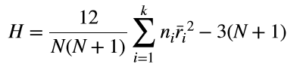

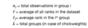
The statistic H is quite easy to compute. The rank represents the position of an item when all items are sorted in ascending order, e.g., r1 represents the smallest value in the set of values. We can see that the statistic is computed from the “ranks” of values in different groups and hence the name Kruskal Wallis “rank” test. The above expression is used if there are no ties in data. In case of ties, a correction is applied to H as follows:
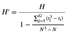
Here ti represents the number of items with the same value having a tie. G is the total number of unique items that have ties. You can see this worked out example for computing H and its correction H’.
To run the test in R, type at the console:
> kruskal.test(weight~feed,data=chickwts)Kruskal-Wallis rank sum test
data: weight by feed
Kruskal-Wallis chi-squared = 37.343, df = 5, p-value = 5.113e-07Step 3: Interpret the result
The distribution of H statistic (or its correction H’) is a chi-square distribution with (k-1) degrees of freedom, where k represents the total number of groups in the data. The H value is used to compute a p-value, which determines if the results are statistically significant. When looking at the p-values, there are different guidelines on when to accept or reject the null hypothesis, (recall from our earlier.discussion that the null hypothesis states that the groups are identically distributed). Generally we compare the p-value with a user defined level of significance denoted by a and make a decision as:
If p > a then accept H0
If p </= a then reject H0 in favor of HA.
The question remains on what should be the value of a. Depending upon your application you can choose a different significance level, e.g., 0.1, 0.05, 0.01 etc.. Michael Baron in his book: “Probability and Statistics for Computer Scientists” recommends choosing an alpha in the range [0.01, 0.1]. So for most applications you can safely accept H0 if p > 0.1 and safely reject H0 if p<0.01. Many scientists set the value of alpha to 0.05 but if your values of p are in the range [0.01,0.1], it may be a good idea to collect more data if your application is a critical one. For the example above we can safely reject the null hypothesis as the p-value is way below 0.1.
Post-hoc test: Applying Wilcoxon rank test
From the above discussion we see that the groups of chicken being fed different types of feed have significantly different distribution of weights. Kruskal Wallis test tells us that at least one group is different, however, it does not tell us which group is different. We require further analysis and need to apply further tests to see which pairs of groups are significantly different from each other, so we will use a Wilcoxon rank sum test. In statistical literature, we call this a post-hoc test.
At the R prompt type (the exact=F parameter indicates that tied ranks are allowed):
> pairwise.wilcox.test(chickwts$weight,chickwts$feed,exact=F)You will see the following output:
Pairwise comparisons using Wilcoxon rank sum test
data:chickwts$weight and chickwts$feed
          casein horsebean linseed meatmeal soybean
horsebean 0.0027 -         -       -        -
linseed   0.0122 0.0644    -       -        -
meatmeal  0.3622 0.0091    0.2181  -        -
soybean   0.0474 0.0091    0.7100  0.7100   -
sunflower 1.0000 0.0017    0.0032  0.3472   0.0140

P value adjustment method: holm
This is a nice and interesting result for different pairs of groups. We can see that many pairs, e.g., (casein, horsebean), (linseed,sunflower), etc. have very low p-values, leading us to conclude that the data provides sufficient evidence that these pairs are different.
Further Readings
I hope you enjoyed this tutorial. R Documentation gives the following book reference in their documentation for Kruskal Wallis test: “Nonparametric Statistical Methods” by Hollander, Wolfe and Chicken. It s a really good reference for further reading and has excellent worked out examples for various statistical tests.
About The Author
Mehreen Saeed is an academic and an independent researcher. I did my PhD in AI in 1999 from University of Bristol, worked in the industry for two years and then joined the academia. My last thirteen years were spent in teaching, learning and researching at FAST NUCES. My LinkedIn profile.