Businesses often need to conduct something called an RFM analysis because of the fact that most businesses obtain 80% of their revenue from just 20% of their customers. Why is this fact relevant? It is the idea upon which an RFM analysis is built. Before I dive into how you can conduct an RFM analysis using R, I’ll explain what exactly it is and why it is needed.
What Is An RFM Analysis?
RFM means recency, frequency and monetary, it measures how much one customer contributes to a business. Recency tells when the most recent purchase of a particular customer was, frequency measures how frequently a customer buys from the business and monetary measures how much a customer spends at the business on average.
RFM analysis was informally introduced by email marketers to target customers individually depending on how they contributed to the business, however, it slowly grew to be an important aspect of customer relationship management for businesses. With a large number of software coming around for customer relationship and specialized marketing, RFM analysis plays an important role in dictating how each customer is to be approached.
Usually, an RFM analysis helps businesses segregate customers into 5 categories of each component, where one category differs from another depending on the contribution of the customer for that particular component. Usually, this is done by assigning the customers a score between 1 and 5 for each component of RFM. 1 is the lowest and 5 is the highest. If a customer buys a water bottle from a business every day then the customer would have an R and F value of 5 whereas the M value would be close to 1. The overall rank of such a customer would be 551. An ideal customer would have a code of 555 whereas a code of 111 would be least ideal. Sometimes, if the business data is smaller, the analyst may rank each category between 1 and 3. In this case an ideal score would be 333.
Analysts most commonly use Excel to conduct an RFM analysis but with the advent of newer and more powerful, and even more specialized tools and software, there are many other ways to go about an RFM analysis. R is one of the most powerful platforms for such business applications. In this tutorial, I will be going over techniques in R that you can use to conduct a quick RFM analysis for your business.
Once you obtain the RFM ranks for all your customers, you can calculate an RFM score. An RFM score of a customer is the aggregate of individual ranks. It tells you the “quality” of a single customer, or the overall quality of the customers visiting your store.
The aggregate score of a customer with an RFM of 555 would be 5 whereas that of a customer with an RFM of 115 would be 2.3. This immediately tells you which customer is more beneficial for your business currently and which customer would respond more to promotional activities.
Why Is An RFM Analysis Required?
Now it may be common to think of RFM as something that is intuitive and does not require a specialized analysis, however, businesses can make a large difference in how effective their marketing strategies are through the use of an RFM analysis.
Normally, there is a very small fraction of the customers who actually respond to promotions and advertisements of businesses. Through an RFM analysis, you understand what to present to a specific customer in the ads and promotions so that you can maximize interaction and response from them. This said, an RFM analysis, in one way, tells you what kind of potential lies in each customer and what interests them. Using RFM to decide your marketing strategies is an effective implementation of data driven marketing.
For example, customers with an RFM rank of 115 would require that you show them promotions and ads that bring them more often to your store. Alternatively, a score of 115 may also tell you that this particular segment of customers would respond more effectively to marketing strategies that describe an incentive of visiting your store. You would know that entering such customers into a loyalty program would be more beneficial for your business as compared to entering a customer with an RFM score of 441.
Customer Segmentation Using RFM Scores
Effective customer segmentation that is defined by the RFM score can be implemented in a number of ways, however, the exact implementation of this segmentation largely depends on the type of business you run. Here are a few categories that generally work for most businesses.
First Grade
The customers who shop from your store very frequently and spend big amounts on each visit. These customers are the first to try out any new additions to your business and would contribute towards the promotion of your business.
Potentially Loyal
These are the customers who aren’t showing up at your store very frequently, but they are heavy spenders. Such customers, as discussed earlier, are potential members of your loyalty program. If your business has many such customers but does not offer a loyalty program, it may be an indication that you need to start one.
Can’t Lose Them
These would be the customers who used to spend large sums of money at your store, but you haven’t seen them in a while. Such a situation requires you to make an effort to bring them back. This may require a completely dedicated advertisement or reconnection strategy.
The number of segments you can fit your customers into is not limited to these, but these are usually the most basic categories that work out for almost all businesses.
How to Conduct An RFM Analysis In R
Now that you are acquainted with what an RFM analysis is and why your business needs one, I can move on to explaining how you can conduct one using R. At first, this may seem like a tedious task that requires extensive scripts written to segregate customer information. Fortunately, R gives you a way around all the hassle. The “rfm” package, for instance, gives you an efficient workaround. The “rfm” package uses data that can be characterized as “customer” or “transaction” and generates an RFM report. For most businesses, the POS system usually records one of these kinds of data, therefore the package can be widely used.
If you haven’t installed the package yet, you can do that using the “install.packages()” command.
> install.packages("rfm")Running an RFM analysis on your data using the “rfm” package requires that you have developer tools set up in your environment. If you haven’t already installed the developer tools, you can do that and load the “rfm” package in the environment using the following code.
> install.packages("devtools")
> library ("rfm")
Now that your environment is all set, we can begin the analysis. In this tutorial I will be using a dataset, “rfm_data_orders” that comes with the “rfm” package as a sample. The dataset contains a unique identification number for customers along with their date of purchase and spending. You can create an RFM analysis report using the “rfm_table_order()” function that comes in the “rfm” package.
The “rfm_table_order()” function takes 8 arguments, that are needed for the report generation.
- The Data: As mentioned above, it should hold information for customer identification, date and monetary value of the transaction.
- Customer ID: This column holds customer identification information.
- Date: It gives the date for each purchase.
- Transaction Amount: Gives the monetary value of each transaction.
- Date of the Analysis: The date relative to which you want the recency to be calculated.
- R Bins: The scale on which recency is calculated.
- F Bins: The scale on which frequency is calculated.
- M Bins: The scale on which the monetary value is calculated.
The last three parameters are set to 5 by default, however, you can tweak that depending on how spread out your data is in terms of these parameters. You need to specify the current date for the report to be generated, it is needed to estimate the relative recency of each individual customer. In the code below, I have added a date of 2006 since the data has been collected up till 2006.
> date <- lubridate::as_date("2006-12-31", tz = "UTC")With all the parameters specified, you are good to plug things into the “rfm_table()” function for generating a report. The RFM report is generated as a table, I will therefore store the analysis in a variable named “report”.
> report <- rfm_table_order(rfm_data_orders, customer_id, order_date, revenue, date)
> report
Upon viewing, your report looks like this.
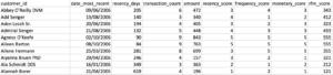
[Here you can see the report that we just generated using our test data, it is important to know what each column represents. “date_most_recent” shows when the last transaction was carried out by a customer, and the “recency_days” column shows how many days it has been since their last visit to the store. “transaction_count” gives a count for the customer’s purchases.
The next three columns give you the rank for recency, frequency and monetary given to each customer by your algorithm. Finally, the last column gives you a consolidated RFM score. It is usually a good idea to save this information in your computer for later use in case you have to come back to it, it should save you a great amount of time.
> write.csv (report$rfm,"Path for where to save file", row.names = FALSE)Customer Segmentation
Customer segmentation tells you precisely how many customers are contributing to your business in what ways and this makes it an important component of the overall analysis.
As said earlier, you define the segments into which your customers are to be divided depending on their RFM score. The data being used here is ideally broken down into the segments as defined below.
> report <- rfm_table_order(rfm_data_orders, customer_id, order_date, revenue, date)
> segment_titles <- c("First Grade", "Loyal", "Likely to be Loyal",
+   "New Ones", "Could be Promising", "Require Assistance", "Getting Less Frequent",
+   "Almost Out", "Can't Lose Them", "Don’t Show Up at All")
After defining the segments, I give a numerical threshold for each component of RFM that categorizes customers in the segments.
> r_low <- c(4, 2, 3, 4, 3, 2, 2, 1, 1, 1)
> r_high <- c(5, 5, 5, 5, 4, 3, 3, 2, 1, 2)
> f_low <- c(4, 3, 1, 1, 1, 2, 1, 2, 4, 1)
> f_high <- c(5, 5, 3, 1, 1, 3, 2, 5, 5, 2)
> m_low <- c(4, 3, 1, 1, 1, 2, 1, 2, 4, 1)
> m_high  <- c(5, 5, 3, 1, 1, 3, 2, 5, 5, 2)

> divisions<-rfm_segment(report, segment_titles, r_low, r_high, f_low, f_high, m_low, m_high)

> library(dplyr) # required for grouping

> divisions %>% count(segment) %>% arrange(desc(n)) %>% rename(Segment = segment, Count = n)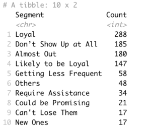
[This gives you a numerical count for customers that lie in each segment that we defined.
Analysis of the Customer Segmentation
Now that you have successfully categorized the customers into segments, you can begin with an analysis of this segmentation. Some of the most common analysis methods have been listed below.
R Median
> rfm_plot_median_recency(divisions)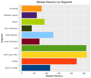
[
F Median
> rfm_plot_median_frequency(divisions)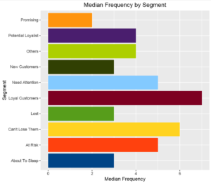
[
M Median
> rfm_plot_median_monetary(divisions)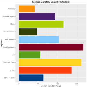
[Put M med here]
RFM Histogram
A histogram is a great way to visualize the results that you obtain from your analysis. The package I have used in this tutorial fortunately gives you a function to do this quickly by only plugging in your results’ data frame as the argument.
> rfm_histograms(report)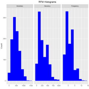
[Put histogram here]
Bar Plot for Orders
Another interesting analysis method is the use of a bar plot to visualize how many purchases customers generally make from your store. The distribution for such data is usually normal.
> rfm_order_dist(report)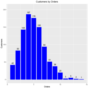
[