A Not-So Naive ‘Naive Bayes’ In R

In this tutorial, I will present a probabilistic algorithm, for classifying data, called the naive Bayes’ algorithm. I say it is not so naive because, despite its simplicity it can be applied successfully to a wide range of problems in data science, machine learning and natural language processing. To keep things simple, I will show you how naive Bayes’ classiﬁer works for binary data for a two class problem. With a good understanding of the working of this algorithm for a two class problem, it can be extended to categorical as well as continuous data for multiple classes.

A Bit Of History

First let us trace the history of this algorithm. Here is a link to Thomas Bayes, who I would say is a super star of data science. Two years after his death an article with the following title was published in 1763:

An Essay Towards Solving A Problem In The Doctrine Of Chances

This was a marvelous piece of work on probability theory and I only wish Bayes knew what a tremendous impact this paper would have on data science and many other ﬁelds. Here I would show (in the simplest possible way) how we can apply Bayes’ theorem to a classiﬁcation problem. Bayes’ theorem is given by:

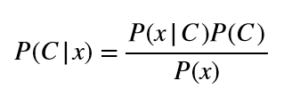
Here C is a variable denoting a class, x is a feature vector. We’ll use x to denote a feature vector and xi to denote an individual feature. We say that P(C|x) is the posterior probability of a class given x, P(C) is the class prior, P(x|C) is the likelihood of data and P(x) is the evidence. In very simple words, the above mathematical formula shows us how we can update the probability of a class (in other words make conclusions about a class) when given the evidence (which is a data point). The class with the highest posterior probability is the predicted class in a classiﬁcation problem.

From Bayes to Naive Bayes

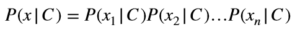
The only problem we face when practically applying Bayes’ theorem is the computation of P(x|C), which may require loads and loads of data for training. We make a simplifying assumption to compute P(x|C) and hence the name “naive Bayes”. Naive Bayes’ assumption is that features are independent given a class variable and we can state it mathematically as:

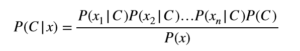
And hence Bayes’ theorem leads to a naive Bayes’ algorithm for computing posterior probability of a class as:

A Simple Example

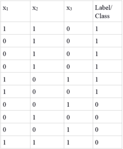
Before implementing this algorithm in R, let us take a very simple example to see how we apply naive Bayes’ for predicting which class, a given data point belongs to. The table below shows 10 training points, which we will use for building our model. Here we have three features and two classes. As this is binary data, we’ll use the symbols ~C for C=0 and C for C=1. Similarly, we’ll use ~xi for xi=0 and xi for xi=1. From the rules of probability we know that: P(~C) = 1-P(C) P(~xi|C) = 1-P(xi|C)

Training Points

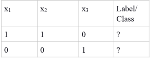
Test points

Training Phase For Our Simple Example

The training phase is quite simple. All we need is P(xi|C) for all features, i.e., for i ={1,2,3} and P(C).

P(x1|C) = 3/6, P(x2|C) = 4/6, P(x3|C) = 1/6

P(x1|~C) = 1/4, P(x2|~C) = 2/4, P(x3|~C)=3/4

P(C) = 6/10

I have not simpliﬁed the fractions deliberately, so that you can see how these values are computed.

Test Phase For Our Simple Example

Now let us apply the mathematical model to determine the class of the test point. Here, I show you the computation for the ﬁrst test point (1,1,0) and you can do it equivalently for the second test point.

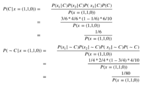
Our predicted class is then Class 1 as the posterior for this class is higher than the posterior for Class 0. Note, we do not have to compute the evidence P(x=(1,1,0)), as it is the same for both classes and does not play a role in classifying a test point.

Our Simple Example In R

Now let us build the framework for implementing our simple example in R. We need to implement the training phase as well as the test phase. During training we need the priors of both classes along with P(xi|C) and P(xi|~C) for each feature. The code we write should be ﬂexible enough to cater for any set of features, whether 3 or 500 or even a million. So we can store P(x|C) as a vector. Also, note that even though we can
directly derive P(~x|C) from P(x|C), most software packages store this parameter to speed up computations in the test phase.

The code for generating the mathematical naive Bayes’ model in R is given below. Since we are using binary data, getting the relative frequency of ones in a class is equivalent to taking column means by using R’s built in colMeans.

trainModel = function(trainData,labels){
#get the indices of the class 1 and class 0
class1 = labels==1
class0 = labels==0
#get the subset of data points for class 1 and class 0 respectively
dataClass1 = trainData[class1,]
dataClass0 = trainData[class0,]
#get  P(x|C)
probxClass1= colMeans(dataClass1)
probxClass0 =colMeans(dataClass0)
#get  P(~x|C)
probNotxClass1 = 1-probxClass1
probNotxClass0 = 1-probxClass0
#getP(C)
priorClass1 = mean(labels)
priorClass0 = 1-priorClass1
return (list(probxClass1=probxClass1, probxClass0=probxClass0, probNotxClass1=probNotxClass1, 
             probNotxClass0=probNotxClass0, priorClass1=priorClass1, priorClass0=priorClass0))
}

The code for the test phase is also given. All that is needed is the computation of the posterior of each class to determine our predicted class.

test = function(x,trainModel){
  #ﬁrst create matrix of prob same size as dat
  r=nrow(x)
  c=ncol(x)
  
  probxClass1<-matrix(rep(trainModel$probxClass1,r),nrow=r,ncol=c,byrow=TRUE)
  probxClass0<-matrix(rep(trainModel$probxClass0,r),nrow=r,ncol=c,byrow=TRUE)
  probNotxClass1<-matrix(rep(trainModel$probNotxClass1,r),nrow=r,ncol=c,byrow=TRUE)
  probNotxClass0<-matrix(rep(trainModel$probNotxClass0,r),nrow=r,ncol=c,byrow=TRUE)
  
  #for class 1
  ind = x==1
  class1Matrix <- x
  class1Matrix[ind]=probxClass1[ind]
  class1Matrix[!ind]=probNotxClass1[!ind]
  
  #for class 0
  class0Matrix <- x
  class0Matrix[ind]=probxClass0[ind]
  class0Matrix[!ind]=probNotxClass0[!ind]
  
  class1Pred = apply(class1Matrix,1,prod)*trainModel$priorClass1
  class0Pred = apply(class0Matrix,1,prod)*trainModel$priorClass0
  
  class1Posterior = class1Pred/(class1Pred+class0Pred)
  class0Posterior = class0Pred  /(class1Pred+class0Pred)
  
  return(list(class1Posterior=class1Posterior,
              class0Posterior=class0Posterior,
              label=class1Pred>=class0Pred))
}

The code for the test phase is quite simple. I explain it for predicting class 1 only. class1Matrix stores the probability P(xi|C) in its corresponding location of the matrix. A step by step guide is given below:

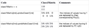
Next we have the following line of code:

class1Pred = apply(class1Matrix,1,prod)*trainModel$priorClass1

This line takes the product of each element in a row and then multiplies it by the prior of that class. The function returns the posterior of the two classes as well as a variable called label, which would be TRUE if class 1 is predicted and FALSE if the predicted class is class 0. A very important thing to note here is that we accomplished everything without using any loops or iterations. By doing the proper math, we can implement lots of data science algorithms without writing very complicated code.

Next we talk about implementation issues and how to deal with them for practical applications, where the dataset might be huge with tons of training and test points.

Practical Considerations: Taking Logarithms

All goes ﬁne when working with naive Bayes’ as illustrated in our code. However, note that the probability of each feature is less than one. When taking products of values less than one, the overall value of P(x|C) becomes very small. For a large number of features you will run into underﬂow errors, either leading to values such as NaN or zero. We can overcome this problem by taking logarithms and noting that:
log(ab) = log(a)+log(b)

Hence, we can compute log(P(C|x)) instead of P(C|x). Our predicted class would then be the class with a higher value of log((PC|X)).

Note again that ln(P(x)) does not play a role in deciding the class for a test point, but when writing math expressions, you must include it. Here I am using natural logarithms but you can use the logarithm with any base. Now the modiﬁed code for the training phase is given below:

trainModelLog = function(trainData,labels){
  
  #get the indices of the class 1 and class 0
  class1 = labels==1
  class0 = labels==0
  
  #get the subset of data points for class 1 and class 0 respectively
  dataClass1 = trainData[class1,]
  dataClass0 = trainData[class0,]
  
  #get  P(x|C)
  probxClass1= colMeans(dataClass1)
  probxClass0 =colMeans(dataClass0)
  
  #get  P(~x|C)
  probNotxClass1 = 1-probxClass1
  probNotxClass0 = 1-probxClass0
  
  #get log(Px|C)
  probxClass1 = log(probxClass1)
  probxClass0 = log(probxClass0)
  
  #get  log(P(~x|C))
  probNotxClass1 = log(probNotxClass1)
  probNotxClass0 = log(probNotxClass0)
  
  #getP(C) and P(~C)
  priorClass1 = mean(labels)
  priorClass0 = 1-priorClass1
  
  #getlog(P(C)) and log(P(~C))
  priorClass1 = log(priorClass1)
  priorClass0 = log(priorClass0)
  
  return (list(probxClass1=probxClass1, probxClass0=probxClass0, probNotxClass1=probNotxClass1, 
               probNotxClass0=probNotxClass0, priorClass1=priorClass1, priorClass0=priorClass0))
}

The modiﬁed code for the test phase is given below. Note the only difference in the test and testLog functions is that we are summing in case of log. Also, the function is returning class1Pred and class0Pred, which are the terms not involving the evidence P(x), i.e., class1Pred is simply computing the following:

ln(P(x1|C))+ln(P(x2|C))+…+ln(P(xn|C))+ln(P(C))

testLog = function(x,trainModel){
  #ﬁrst create matrix of prob same size as dat
  
  r=nrow(x)
  c=ncol(x)
  
  probxClass1<-matrix(rep(trainModel$probxClass1,r),nrow=r,ncol=c,byrow=TRUE)
  probxClass0<-matrix(rep(trainModel$probxClass0,r),nrow=r,ncol=c,byrow=TRUE)
  probNotxClass1<-matrix(rep(trainModel$probNotxClass1,r),nrow=r,ncol=c,byrow=TRUE)
  probNotxClass0<-matrix(rep(trainModel$probNotxClass0,r),nrow=r,ncol=c,byrow=TRUE)
  
  #for class 1
  ind = x==1
  class1Matrix <- x
  class1Matrix[ind]=probxClass1[ind]
  class1Matrix[!ind]=probNotxClass1[!ind]
  
  #for class 0
  class0Matrix <- x
  class0Matrix[ind]=probxClass0[ind]
  class0Matrix[!ind]=probNotxClass0[!ind]
  
  class1Pred = apply(class1Matrix,1,sum)+trainModel$priorClass1
  class0Pred = apply(class0Matrix,1,sum)+trainModel$priorClass0
  
  return(list(class1Pred=class1Pred,class0Pred=class0Pred,
              label=class1Pred>=class0Pred))
}

Smoothing Probability Estimates

We are almost done with a practical implementation of naive Bayes’ classiﬁer for binary classiﬁcation. The only problem left for us to handle is when our training point has no occurrence of a certain value. Imagine an entire feature having only ones and not a single zero for a particular class. This would mean that P(xi|C) is zero, hence reducing the posterior of that class to zero and the entire model collapses. The example below illustrates an instance of this problem, where I have added a fourth feature x4:

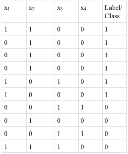
We can see that feature 4 has only zero values in class 1, giving us P(x4=1|C)=0. There are several ways of dealing with this issue, and in case of naive Bayes’ we can obtain smoothed estimates of probability. Even if you do not have the above mentioned problem in your dataset, I still recommend smoothing your probability estimates as it produces great results. We can obtain a smoothed estimate of probability by using the following expression:

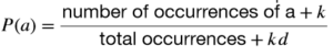
Here k is called the smoothing parameter and you can set it to diﬀerent values.
When k = 0, no smoothing takes place and we have raw estimates of probability. Everything works as mentioned in our examples above. When k>0, we get smoothed estimates. My advise is to use k =1, which is a special type of smoothing called Laplacian smoothing. The variable d in the expression above represents the total number of diﬀerent values of a. So in our case of binary numeric variables and binary classes d = 2. Let us repeat the training phase by applying Laplacian smoothing to compute probability estimates.
P(x1|C) = (3+1)/(6+2) = 4/8, P(x2|C) = (4+1)/(6+2)=5/8, P(x3|C) = (1+1)/(6+2)=2/8, P(x4|C) = (0+1)/(6+2)=1/8 Similarly for class = 0, we get: P(x1|~C) = 2/6, P(x2|~C) = 3/6, P(x3|~C)=4/6, P(x4|~C)=3/6 Similarly the priors are: P(C) = 7/12 P(~C) = 5/12

One important point to note here is that there is a considerable difference between our smoothed and raw (un-smoothed) estimates of probability. This would be true whenever your total sample points are very small in number. For bigger sets (for example 1000 or more), the smoothed estimates would be very close to the raw estimates.

Here is the modiﬁed training phase that incorporates logarithms as well as Laplacian smoothing for probability estimates:

trainModelLogSmooth = function(trainData,labels){
  
  #get the indices of the class 1 and class 0
  class1 = labels==1
  class0 = labels==0
  
  #get the subset of data points for class 1 and class 0 respectively
  dataClass1 = trainData[class1,]
  dataClass0 = trainData[class0,]
  
  #get  P(x|C) and P(x|~C) via Laplacian smoothing
  probxClass1= (colSums(dataClass1)+1)/(nrow(dataClass1)+2)
  probxClass0= (colSums(dataClass0)+1)/(nrow(dataClass0)+2)
  
  #get  P(~x|C)
  probNotxClass1 = 1-probxClass1
  probNotxClass0 = 1-probxClass0
  
  #get log(Px|C)
  probxClass1 = log(probxClass1)
  probxClass0 = log(probxClass0)
  
  #get  log(P(~x|C))
  probNotxClass1 = log(probNotxClass1)
  probNotxClass0 = log(probNotxClass0)
  
  #getP(C) and P(~C)
  priorClass1 = (sum(labels)+1)/(length(labels)+2)
  priorClass0 = 1-priorClass1
  
  #getlog(P(C)) and log(P(~C))
  priorClass1 = log(priorClass1)
  priorClass0 = log(priorClass0)
  
  return (list(probxClass1=probxClass1, probxClass0=probxClass0, probNotxClass1=probNotxClass1, 
               probNotxClass0=probNotxClass0, priorClass1=priorClass1, priorClass0=priorClass0))
}

The test phase remains as it was before.

Putting It All Together

Here is the script you can run in R that makes a call to load the data ﬁle, build a model and then use the model to ﬁnd predictions for the test points. You can download the training data trainSimple1.txt and testSimple1.txt, which contain 4 features or you can use trainSimple.txt and testSimple.txt with 3 features.

Download

You can play around with this code and look at the various parameters being stored in naiveModel. The ﬁnal prediction for each class can be viewed by looking at predict$label.

About The Author

Mehreen Saeed is an academic and an independent researcher. I did my PhD in AI in 1999 from University of Bristol, worked in the industry for two years and then joined the academia. My last thirteen years were spent in teaching, learning and researching at FAST NUCES. My LinkedIn profile.