R’s Favorite: Nearest Neighbors

In this tutorial, I will talk about the awesome k nearest neighbor and its implementation in R. The k-nearest neighbour algorithm, abbreviated k-nn, is surprisingly simple and easy to implement, yet a very powerful method for solving classiﬁcation and regression problems in data science. Here, in this tutorial, I will only talk about the working of knn in r as a classifier but you can easily modify it to implement a predictor for regression problems.

How K-nn Works

In machine learning algorithms, the knn algorithm belongs to the class of “lazy” learners as opposed to “eager” learners. The terminology is quite suitable to describe this classifier as it does nothing during the training phase and applies its predictive abilities only at the test phase. So you need to store all the training points along with their labels in a smart way and use them to classify points during the test phase. In general, k-nn works with numeric variables rather than categorical variables.

You can think of k-nn’s working as similar to a social network or a society, where people who are closest to us (in terms of relationships at work or home) inﬂuence us the most. To see how the knn function works, I have constructed a very simple example with just two classes. See the figure below, where there are points in 2D space and each point belongs to either the green class or the blue class:

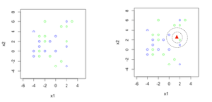
Figure 1: Training points Figure 2: Training points (green+blue) and the test point (red triangle)

In the Figure 2, I have a test point, represented by a red triangle, whose class is unknown and our classifier has to decide its label. Think of the red triangle as a boat. The fisherman inside the boat throws a magic net around it and keeps growing the net till it catches k training points (instead of fish). The label of the majority training points is the predicted label. In Figure 2, if k is set to 1, then a green training point is caught and the prediction is green. If k=3, a bigger net is required and the prediction is blue, as out of the three caught training points, two are blue and one is green. The variable k, is therefore, a user defined parameter, and it speciﬁes how many closest neighbors to look at for deciding the class of a test point. Normally, for a two class problem we set k to an odd number (e.g., 1,3,5,…), to avoid ties between classes.

k-nn is as simple as that. All you need to ﬁgure out is a way to know which are the closest neighbors. You can use any distance measure you like. The most popular is euclidian distance but there is nothing stopping us from using other distance measures like Manhattan distance or a more general Minkowski distance. You can even use similarity measures like Jaccard index or cosine similarity etc., depending on the nature of the data you have at hand. In this tutorial, I’ll show you the working of k-nn, implemented using Euclidean distance. The distance between two points a and b is given by:

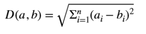
Here a and b are n-dimensional points and ai and bi in the square root represent ith feature for a and b respectively

K-nn In R

Lets do a straightforward and easy implementation in R. As long as we have a distance function in R we can implement k-nn in a data set or data frame. Given below is my implementation of Euclidean distance in R.

Euclidean distance in R

The R function called “euclideanDistance” takes a point and a data matrix as parameters and computes the Euclidean distance between the point and each point of the data matrix. Of course, for this to work correctly the dimensions of all data points should be the same.

#function to return Euclidean distance between a point and points stored in matrix dat
#both pt and dat should have the same dimensions
#pt is then 1xn and dat is mxn
#return would be a vector of m values indicating distance of pt with each row of dat
euclideanDistance <-function(pt,dat)
{
   #get the diﬀerence of each pt's value with dat
   #as R treats data column by column we take the transpose of dat and then transpose again
   #to make sure a vector (pt) is substracted row by row from dat
   diﬀ = t(pt-t(dat))
   #get square of diﬀerence
   diﬀ = diﬀ*diﬀ
   #add all square of diﬀerences
   dist = apply(diﬀ,1,sum)
   #take the square root
   dist = sqrt(dist)
   return(D=dist)
}

In the code above “pt” is a single vector of values and “dat” is a matrix. For example suppose:
pt = (1,2)
dat has two points: ((3,2),(5,5))
The Euclidean distance is then computed as:
Distance between (1,2) and (3,2) = sqrt((1-3)(1-3)+(2-2)(2-2)) = sqrt(4) = 2
Distance between (1,2) and (5,5) = sqrt((1-5)(1-5)+(2-5)(2-5)) = sqrt(25) = 5
The function, hence, returns the vector (2,5) indicating the distance of pt with each row of dat.

R is awesome when it comes to computing with vectors and matrices. Note, we did not use any loops for implementing the above. The code is pretty straightforward except maybe the line that takes the diﬀerence of values of the point pt with all points of the matrix dat:

diﬀ = t(pt-t(dat))

You may wonder why I have used the transpose function t() here. To take the diﬀerence of the point with all points of the data matrix, a simple command such as “diﬀ=pt-dat” won’t work. To subtract a matrix from a point, R makes duplicate copies of pt as (1,2,1,2) to match the size of dat. It also stores dat as a vector in column major order, making its vector representation: (3,3,2,6)

If we do a simple diﬀerence as:

wrongDiﬀ = pt-dat

Then wrongDiﬀ has (1-3,2-3,1-2,2-6), giving us the wrong result (we need (1-3,2-2,1-5,2-5). To make a correction, we subtract pt from dat in row major order by taking the transpose of dat (hence the command (pt-t(dat)). Transpose it back again to get the original matrix dimensions:

diﬀ = t(pt-t(dat)).

Mode in R

The next module we need is a function that computes the mode of a vector. The mode is a statistical function that returns the most frequently occurring values in a list. We need the mode to decide the class of a point, when given the k closest training points. As shown in the earlier example, for 3-nn if the nearest points are (green, blue, blue) then mode would return blue. Unfortunately, R does not have a built in function to compute the mode of a list of values so let’s write our own code to do it. The code below computes the mode:

#get the mode of a vector v
modeValue <- function(v)
{
  if (length(v)==1) 
    return(v)
  #construct the frequency table
  tbl = table(v) 
  #get the most frequently occurring value 
  myMode = names(tbl)[which.max(tbl)]
  return (myMode=myMode)
}

The “table” function returns frequencies of each value in v. Try it at your end as given in the screen shot below, where the table command returns a nice summary of values in v:

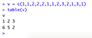
In the next line:

myMode = names(tbl)[which.max(tbl)]

which.max(tbl) returns the index of maximum value and names() returns its value.

K-nn: Putting It All Together

Now we are ﬁnally ready to implement k-nn. See the code below:

#will apply knn algorithm to ﬁnd the label of the testPoints, when given 
#trainData and corresponding labels
#default value of k parameter is 1 and you can pass any distance function
#as a parameter as long as the function has pt and data as parameters
testknn <- function(trainData,trainLabels,testPoints,k=1,distFunc=euclideanDistance)
{
  
  totalTest = nrow(testPoints)
  predictedLabels = rep(0,totalTest)
  for (i in 1:totalTest)
  {
    
     distance = distFunc(pt=testPoints[i,],dat=trainData)
     nearestPts = sort(distance,index.return=TRUE)
     nearestLabels = trainLabels[nearestPts$ix][1:k]
     predictedLabels[i] = modeValue(nearestLabels)
  }
  return(predictedLabels)
}

This code is pretty simple. The parameters for testknn function are the training data points, their corresponding labels, value of k (set to 1 by default) and a distance function, which by default is Eucidean distance. Use the distance function as a function parameter so that later you can write other distance functions and pass them as parameters, without re-writing the whole code for k-nn.

Testknn function takes each point in the test set, computes its Euclidean distance with each training point, sorts the distances and ﬁnds the predicted labels using our implemented mode function. That’s it, we are done writing k-nn code. K-nn being a lazy algorithm puts us programmers at an advantage as there is nothing to do in the training phase (although for huge datasets it’s not true. You may have to apply some smart tricks to extract summaries of data). Now that we have this nice R code lets have some fun with k-nn and see how it works.

Coding For Decision Boundaries In R

When working with any classiﬁer, we are interested in seeing what kind of decision boundaries it makes. For example, logistic regression makes linear decision boundaries and there are some classiﬁers that make nonlinear boundaries (for example neural networks). It’s very easy to visualize the decision boundary for any classiﬁer by taking points in the 2D space. We can treat the points in the entire space as test points, classify them and then plot them in diﬀerent colors according to their classiﬁcation to see which regions belong to which class. For example, if we take the training points as given in Figure 1, then the rest of the points around it form our test set. Classifying them as blue or green will give us an idea of which points belong to the blue class and which of them belong to the green class.

To visualize the decision boundaries in R, ﬁrst we need a small function “plotData” that plots diﬀerent points having the same label in the same color. At the start if newPlot is set to TRUE then a new graphics object is created, otherwise the data is plotted on an older graph. You’ll see its usefulness later. The “unique” function gives us all the unique labels without duplicates and “points” function is called for each label in a for loop. Note the default value of style in the “points” function is set to 1, which are open circles.

#plot data points with labels in diﬀerent colors
#if you have more than 4 labels then send the colors array as parameter with more colors
plotData <- function(dat,labels,colors=c('lawngreen','lightblue','red','yellow'),newPlot=TRUE,style=1)
{
  
  l = unique(labels)
  l = sort(l)
  #initialize the plot if speciﬁed in parameters
  if (newPlot)
    plot(1,xlim=c(min(dat[,1])-1,max(dat[,1])+1),ylim=c(min(dat[,2])-1,max(dat[,2])+1), 
            col=“white", xlab=“x1", ylab="x2")
  count=1
  for (i in l)
  {
      
       ind = labels==i
       points(dat[ind,1],dat[ind,2],col=colors[count],pch=style)
       count = count+1
  }
}

Now let’s code to view the decision boundary of k-nn.

#function to make the decision boundary of k-nn
decisionBoundaryKnn <- function(trainData,trainLabels,k=1)
{
  #generate test points in the entire boundary of plane
  #subtract -2 from in and +2 from max to extend the boundary 
  x1 <- seq(min(trainData)-2,max(trainData)+2,by=.3)
  l = length(x1)
  x2 = x1 
  #this will make x-coordinate
  x1 = rep(x1,each=l)
  #this will make y-coordinate
  x2 = rep(x2,times=l)
  #construct the ﬁnal test matrix by placing x1 and x2 together
  xtest = cbind(x1,x2)
  
  
  predictions=testknn(trainData,trainLabels,testPoints=xtest,k)  
  #plot the test points with predicted labels
  plotData(dat=xtest,labels=predictions)
  #plot the training points in a diﬀerent style (ﬁlled circles)
  plotData(dat=trainData,labels=trainLabels,newPlot=FALSE,style=16,colors=c('green','blue'))
}

The ﬁrst part of the code generates points “xtest” in the entire space, calls the k-nn to classify these points and then calls plotData to plot those points. In the end it also plots the training points but in a diﬀerent color so that we can see the diﬀerence between training and test points. Also, the training points are plotted with style 16, which speciﬁes ﬁlled circles. Lets see this function in action next.

Visualizing Decision Boundaries Of K-nn

Lets look at our simple example given in Figure 1. You can download the sample points knnTrainPoints.txt here{URL needed for ﬁle}. First load the training points in memory by typing the following code:

x=(read.table("knnTrainPoints.txt"))
x=data.matrix(x)
labels = x[,ncol(x)]
x = x[,-ncol(x)]

The graphs in the next sections show the decision boundary, which you can reproduce using the code shown in the box of each plot. The solid circles, which are also the darker points are the training points. The lighter colors are the test points that we generated in the entire space.

Variable Number Of Training Points And Fixed K=1

To see how the decision boundary changes with a change in the number of training points, let’s run the code for 2,4, 10 and all the points. For two training points, we have a linear decision boundary just as expected. The line is equidistant from the two training points. If we are unlucky our test point would fall on that line and we would have a point of confusion as the point could belong to either of the two classes. In this case, just pick a class randomly. This situation would occur rarely in real life applications but it is not impossible.
When two more training points are added, see how the boundary shifts with each point exerting its inﬂuence on the test points. Adding more and more points makes more complex boundaries for k=1.

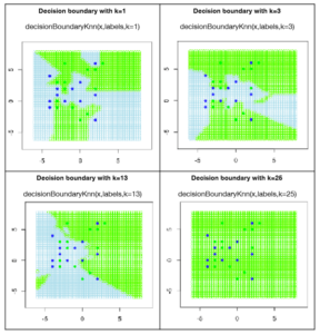
Figure 3: Decision boundaries for variable number of training points and k=1

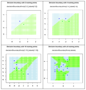
Figure 4: Decision boundaries for variable k

Variable k, Fixed Number Of Training Points

Now lets see what eﬀect the parameter k has on deciding the classiﬁcation of the test points. The correct technical word for k is a hyper parameter (although you can get away by simply saying parameter). For k=1, only the closest point is important and so each training point has its own region of inﬂuence. For higher values of k, many training points together decide the boundary. I deliberately selected 13 green training points and 12 blue ones, making a total of 25 training points. Note what happens when we take k=25 and you can ﬁgure out why all the test points are now classiﬁed as green. You will see that for values of very large values of k, k-nn would start favoring the green class for obvious reasons. Determining which value of k to use is still a challenge and many researchers working in the area of model selection are trying to answer this question.

Applying K-nn For OCR

The application, I have chosen, for applying k-nn, is the recognition of handwritten digits. There is a very nice dataset for OCR at UCI machine learning repository and we thank them for their support. Here is a reference to the repository:

Dua, D. and Graﬀ, C. (2019). UCI Machine Learning Repository [http://archive.ics.uci.edu/ml]. Irvine, CA: University of California, School of Information and Computer Science.

You can download the OCR dataset from the machine learning repository from this link.
The dataset was contributed by Alpaydin and Kaynak and it has pre-processed handwritten images of the digits 0-9. In particular, we’ll work with the training set optdigits.tra and test ﬁle optdigits.tes.

I am pasting here 3 example images from this dataset and you can generate them too using the code I am providing.

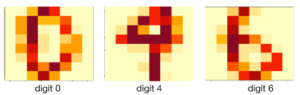
Figure 5: Example images of handwritten digits from UCI machine learning repository

The function “knnOcr” returns the accuracy rate of the classiﬁer. The default value for k is again 1. This function reads the training and test ﬁles, separates their labels and calls the testknn function that we wrote earlier. If you want to view the images of the dataset you can uncomment the lines in the code below.

knnOcr <- function(k=1)
{
  #read the training and test ﬁles and separate their labels
  trainData <- read.csv('digits/optdigits.tra',header = FALSE)
  trainData = data.matrix(trainData)
  trainLabels = trainData[,ncol(trainData)]
  trainData = trainData[,-ncol(trainData)]
  testData  <- read.csv('digits/optdigits.tes',header = FALSE)
  testData = data.matrix(testData)
  testLabels = testData[,ncol(testData)]
  testData = testData[,-ncol(testData)]
  ##########################################################
  #uncomment the following lines if you want to display an image
  #at any index set by indexToDisplay
  #ﬂip image to display properly
  #start uncommenting now
  #indexToDisplay = 1
  #digit = trainData[indexToDisplay,]
  #dim(digit) = c(8,8)   #reshape to 8x8 images
  #im <- apply(digit,1,rev)
  #image(t(im))
  #stop uncommenting now
  ################################################################
  predictions = testknn(trainData,trainLabels,testPoints=testData,k)
  #compute accuracy of the classiﬁer
  totalCorrect=sum(predictions==testLabels)
  accuracy = totalCorrect/length(predictions)
  return(accuracy)
}

Run the following command:
knnOcr()

This would return the number 0.9799666, which shows that the digits were recognized with 98% accuracy rate. That’s simply marvelous! You can run the same function for diﬀerent values of k and see how it goes. This link has information on the accuracy of k-nn classiﬁer for diﬀerent values of k for this dataset. Do run it yourself and verify whether your percentage accuracy matches theirs.

About The Author

Mehreen Saeed is an academic and an independent researcher. I did my PhD in AI in 1999 from University of Bristol, worked in the industry for two years and then joined the academia. My last thirteen years were spent in teaching, learning and researching at FAST NUCES. My LinkedIn profile.